library(here)
library(tidyverse)
df_data <- read_csv(here("data", "steps_clean.csv"))Sampling from a population
So far, we have restricted ourselves to describing the sample that we have. Often, however, we are not only interested about our sample, but want to make inferences about the population from which our sample came.
Load packages and data
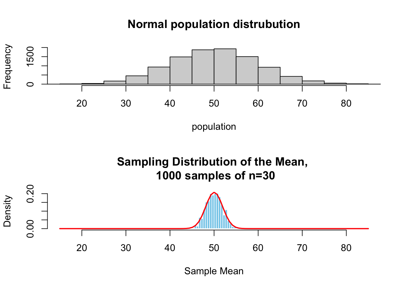
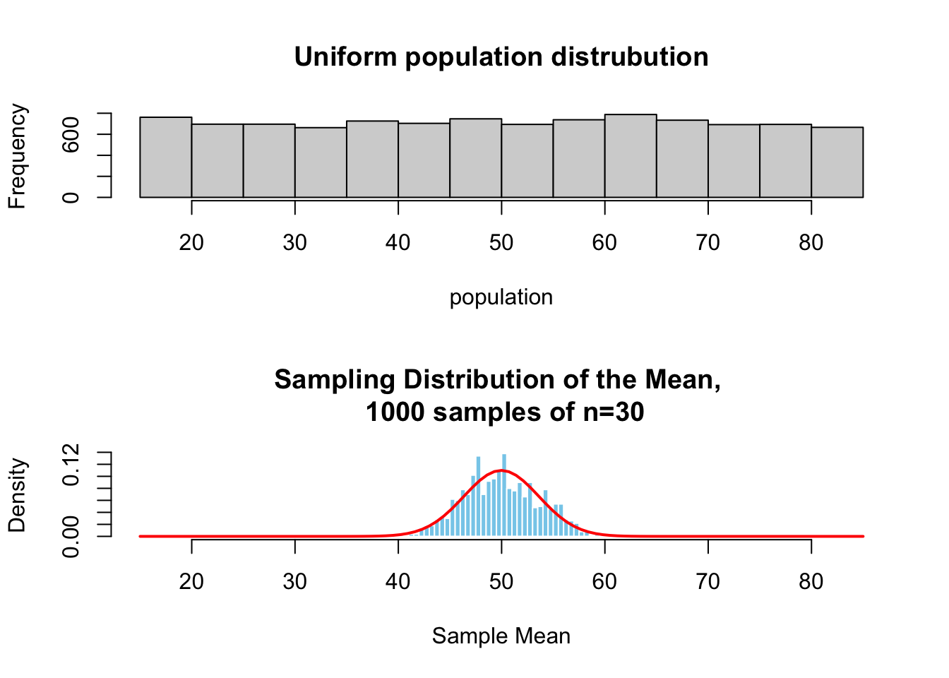
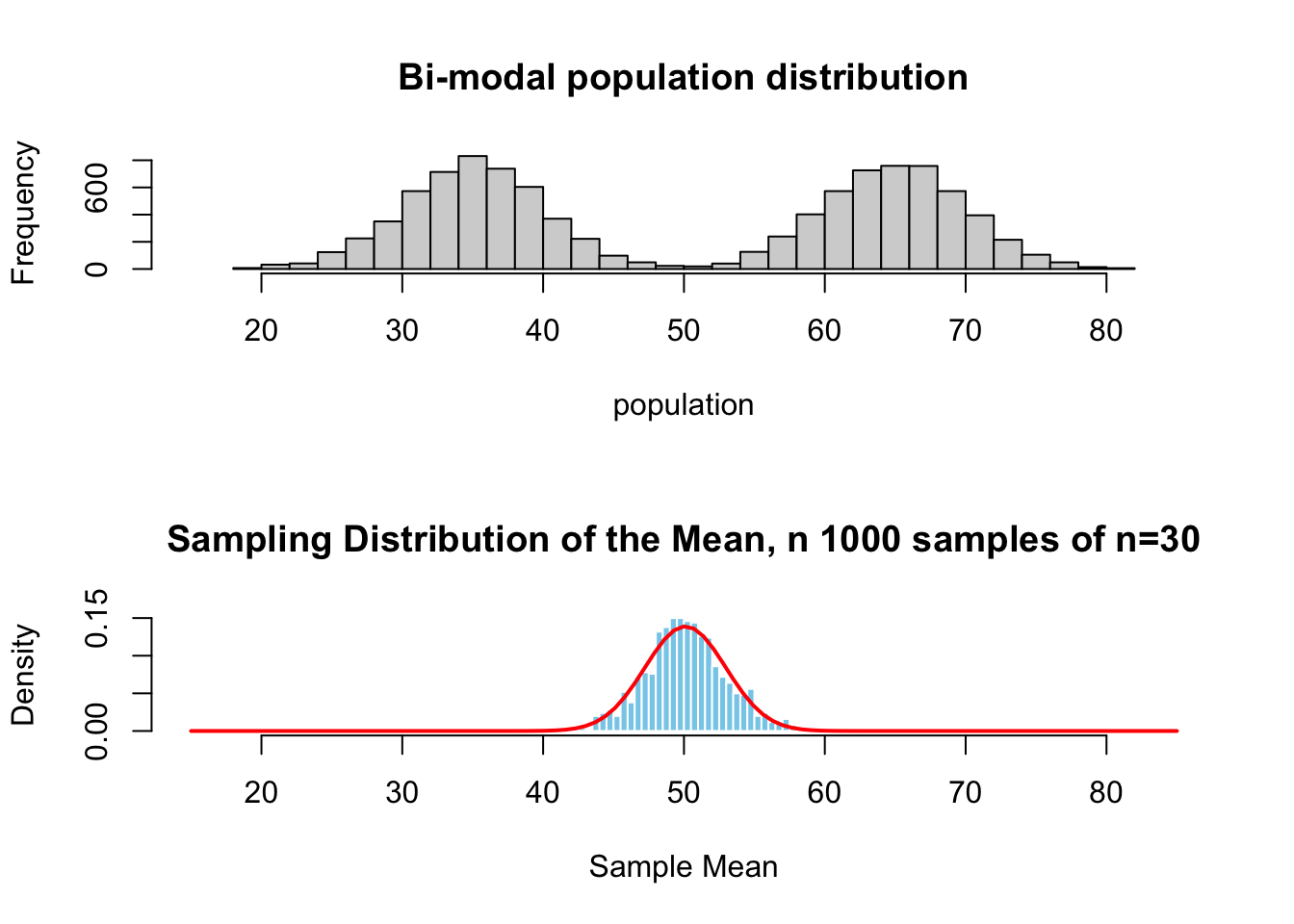
Central Limit Theorem (CLT):
No matter what the population distribution looks like, if you take many random samples and calculate their means, those samples means will form a normal distribution as the sample size grows large.
- Sample means become normally distributed.
- Happens even if the original population is not normal.
- Works better as sample size increases (n ≥ 30 is a common rule).
Here is a simulation to visualize what the relation between the distribution of a variable in the population and the sampling distribution of the means from that same population.
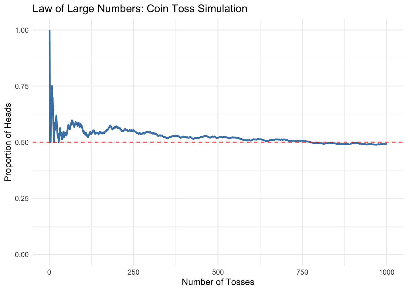
Law of Large Numbers (LLN):
As you collect more and more observations, the sample mean (or proportion) will get closer and closer to the true population mean.
- More data = more accuracy.
- Guarantees that with enough data, random variation averages out.
Imagine that we had the patience to flip a coin 1000 times. For each toss, we calculated the number of heads we’ve gotten so far and divided by the total tosses, to get the proportion that landed heads. Even if we expect the coin to be fair, we wouldn’t expect it to be 50-50 heads and tails in the beginning. In fact, at the first toss that would be impossible, As we continued, however, we would see the proportion of heads gradually stabilize around 0.5.
Together the central limit theorem and the law of large numbers tells us that when sampling from a population 1) the sampling distribution approaches a normal distribution as the number of samples increases, AND 2) the value of the sample mean \(\bar{x}\), the estimate, will approach the true population mean \(\mu\) as the sample size increase.
Sampling in research
This is all fine and well, but you may find yourself wondering “How does this help my PhD?”. You won’t be able to sample repeatedly from the population, if you are lucky you’ll have ONE sample to work with. But there is an upside! You can use you sample values to estimate the standard deviation of the sampling distribution, also known as the standard error (SE).
Standard error of a mean
The formula for the standard error of a mean, if we knew the population variance \(\sigma^2\), is:
\[ SE = {\sqrt{\sigma^2 / n}} \]
However, we rarely know the population standard deviation. Luckily we can use the sample variance \(s^2\) to estimate it:
\[ SE = {\sqrt{s^2 / n}} \]
Base R has no built-in functions for standard errors, but you can easily calculate them from formulas. To calculate the standard error of the LSAS scale at screening, we can use the following code:
sd(df_data$lsas_screen)/sqrt(length(df_data$lsas_screen))[1] 1.224066# or we can create a function
stderr <- function(x) sd(x) / sqrt(length(x))
stderr(df_data$lsas_screen)[1] 1.224066Standard error of a proportion
For a proportion, the standard error for the population is calculated by the formula:
\[ \mathrm{SE}(p) = \sqrt{\frac{p(1 - p)}{n}} \]
We can get this in R using the following code:
# Simulating a gender variable
n <- nrow(df_data)
df_data$gender <- rbinom(n, 1, 0.7)
df_data$gender <- ifelse(df_data$gender == 1, "Woman", "Man")

p <- mean(df_data$gender=="Man") # using the mean function to get the probability
n <- nrow(df_data) # the number of observations (since we have no NA values)
se <- sqrt(p * (1 - p) / n) # standard error
se
[1] 0.03382401