1 Introduction

In the previous chapter, we studied regression models with two binary predictors, and learned how to distinguish between:

additive models (no interaction)
interaction models (effect modification)

In this chapter, we extend these ideas to a model with:

one binary predictor: trt (therapist-guided vs waitlist)
one numeric predictor: phq9_screen (baseline depression severity)

This allows us to introduce conditional effects when the moderator is numeric, and to distinguish between:

parallel slopes (no interaction): the treatment effect is constant across phq9_screen
effect modification (interaction): the treatment effect varies with phq9_screen

You will learn:

how to interpret models with one binary and one numeric predictor
how conditional treatment effects vary across values of a numeric variable
how interactions change interpretation
how to estimate conditional and marginal effects using marginaleffects
how to visualize interactions with predicted values

2 Packages and Data

library(tidyverse)
library(broom)
library(quantreg)
library(marginaleffects)
library(here)

2.1 Load data

df_clean <- read_csv2(here("data", "steps_clean.csv"))

As before, we use treatment group as our binary predictor. We subset the data to include only participants in the therapist-guided and waitlist conditions.

df_red <- filter(df_clean, trt %in% c("therapist-guided", "waitlist"))
df_red <- df_red |> mutate(
  trt = factor(trt, levels = c("waitlist", "therapist-guided"))
)

The other predictor will be baseline depression severity measured continuously using phq9_screen.

summary(df_red$phq9_screen)

   Min. 1st Qu.  Median    Mean 3rd Qu.    Max. 
   1.00    7.00    9.00    9.85   13.00   19.00

3 One Binary and One Numeric Predictor without Interaction (Additive Model)

We begin with a model that includes both predictors without an interaction.

3.1 Model formula

lsas_post ~ trt + phq9_screen

This corresponds to the linear regression model for the conditional mean:

\[ \begin{aligned} \mathbb{E}(LSAS_{post,i} \,\mid\, trt_i,\; phq9\_screen_i) =& \beta_0 + \\ & \beta_1\, \mathbf{1}\{\text{trt}_i = \text{therapist-guided}\} + \\ & \beta_2\, phq9\_screen_i \end{aligned} \]

Where:

\(\beta_0\): mean outcome when trt = waitlist and phq9_screen = 0
\(\beta_1\): conditional treatment effect holding PHQ-9 constant
\(\beta_2\): conditional effect of PHQ-9 holding treatment constant

Interpretation

In this model:

the treatment effect is assumed to be the same at all values of PHQ-9
the PHQ-9 slope is assumed to be the same in both treatment groups

This is an additive model (parallel slopes).

4 Linear Regression without Interaction

4.1 Fit the model

mod_lm_add <- lm(lsas_post ~ trt + phq9_screen, data = df_red)
summary(mod_lm_add)


Call:
lm(formula = lsas_post ~ trt + phq9_screen, data = df_red)

Residuals:
    Min      1Q  Median      3Q     Max 
-65.918 -13.561  -0.148  12.947  62.865 

Coefficients:
                    Estimate Std. Error t value Pr(>|t|)    
(Intercept)          63.3772     5.9399  10.670  < 2e-16 ***
trttherapist-guided -19.3976     4.4906  -4.320 3.46e-05 ***
phq9_screen           1.4617     0.4919   2.972  0.00364 ** 
---
Signif. codes:  0 '***' 0.001 '**' 0.01 '*' 0.05 '.' 0.1 ' ' 1

Residual standard error: 23.55 on 109 degrees of freedom
  (8 observations deleted due to missingness)
Multiple R-squared:  0.2229,    Adjusted R-squared:  0.2086 
F-statistic: 15.63 on 2 and 109 DF,  p-value: 1.074e-06

Interpretation

Intercept: mean LSAS at post when trt = waitlist and phq9_screen = 0
(note: phq9_screen = 0 may be outside the range of the data, so the intercept is often not directly meaningful)
trt coefficient: treatment effect adjusted for PHQ-9
phq9_screen coefficient: association between baseline depression and post-treatment LSAS, adjusted for treatment

4.2 Predicted means for each treatment group (averaged over PHQ-9)

avg_predictions(mod_lm_add, by = "trt")

trt	Estimate	Std. Error	z	Pr(>\|z\|)	2.5 %	97.5 %
Type: response
waitlist	78.4	3.09	25.4	<0.001	72.4	84.5
therapist-guided	57.4	3.21	17.9	<0.001	51.1	63.6

4.3 Treatment effect as a conditional contrast

Because there is no interaction, the conditional treatment effect is the same for all PHQ-9 values.

avg_comparisons(mod_lm_add,
  variables = "trt",
  by = "phq9_screen"
)

phq9_screen	Estimate	Std. Error	z	Pr(>\|z\|)	2.5 %	97.5 %
Type: response
1	-19.4	4.49	-4.32	<0.001	-28.2	-10.6
2	-19.4	4.49	-4.32	<0.001	-28.2	-10.6
3	-19.4	4.49	-4.32	<0.001	-28.2	-10.6
4	-19.4	4.49	-4.32	<0.001	-28.2	-10.6
5	-19.4	4.49	-4.32	<0.001	-28.2	-10.6
6	-19.4	4.49	-4.32	<0.001	-28.2	-10.6
7	-19.4	4.49	-4.32	<0.001	-28.2	-10.6
8	-19.4	4.49	-4.32	<0.001	-28.2	-10.6
9	-19.4	4.49	-4.32	<0.001	-28.2	-10.6
10	-19.4	4.49	-4.32	<0.001	-28.2	-10.6
11	-19.4	4.49	-4.32	<0.001	-28.2	-10.6
12	-19.4	4.49	-4.32	<0.001	-28.2	-10.6
13	-19.4	4.49	-4.32	<0.001	-28.2	-10.6
14	-19.4	4.49	-4.32	<0.001	-28.2	-10.6
15	-19.4	4.49	-4.32	<0.001	-28.2	-10.6
16	-19.4	4.49	-4.32	<0.001	-28.2	-10.6
17	-19.4	4.49	-4.32	<0.001	-28.2	-10.6
18	-19.4	4.49	-4.32	<0.001	-28.2	-10.6
19	-19.4	4.49	-4.32	<0.001	-28.2	-10.6

5 Adding an Interaction

Now we allow the treatment effect to differ depending on baseline depression severity.

5.1 Model formula with interaction

lsas_post ~ trt * phq9_screen

Which expands to the conditional mean:

\[ \begin{aligned} \mathbb{E}(LSAS_{post,i} \,\mid\, trt_i,\; phq9\_screen_i) =& \beta_0 + \\ & \beta_1\, \mathbf{1}\{\text{trt}_i = \text{therapist-guided}\} + \\ & \beta_2\, phq9\_screen_i + \\ & \beta_3\, \mathbf{1}\{\text{trt}_i = \text{therapist-guided}\} \times phq9\_screen_i \end{aligned} \]

\(\beta_3\) is the interaction term, it captures how the treatment effect changes as PHQ-9 increases

We now allow the treatment effect to differ depending on baseline depression, rather than remaining constant across PHQ-9 values.

6 Linear Regression with Interaction

6.1 Fit the interaction model

mod_lm_int <- lm(lsas_post ~ trt * phq9_screen, data = df_red)
summary(mod_lm_int)


Call:
lm(formula = lsas_post ~ trt * phq9_screen, data = df_red)

Residuals:
    Min      1Q  Median      3Q     Max 
-65.585 -13.229  -0.181  13.429  62.900 

Coefficients:
                                Estimate Std. Error t value Pr(>|t|)    
(Intercept)                      65.4083     7.5650   8.646 5.45e-14 ***
trttherapist-guided             -23.5820    10.5995  -2.225   0.0282 *  
phq9_screen                       1.2647     0.6691   1.890   0.0614 .  
trttherapist-guided:phq9_screen   0.4324     0.9913   0.436   0.6636    
---
Signif. codes:  0 '***' 0.001 '**' 0.01 '*' 0.05 '.' 0.1 ' ' 1

Residual standard error: 23.64 on 108 degrees of freedom
  (8 observations deleted due to missingness)
Multiple R-squared:  0.2243,    Adjusted R-squared:  0.2027 
F-statistic: 10.41 on 3 and 108 DF,  p-value: 4.513e-06

Interpretation

The treatment effect is conditional on PHQ-9
Main effects are interpreted at the reference level of the other variable:
- the trt coefficient is the treatment effect when phq9_screen = 0
- the phq9_screen coefficient is the PHQ-9 slope in the waitlist group (reference level)
The interaction coefficient represents how much the treatment effect changes for a one-unit increase in PHQ-9. For example, a negative interaction means the treatment effect becomes more negative (larger improvement) at higher PHQ-9.

6.2 Conditional treatment effects at selected PHQ-9 values

A simple way to interpret the interaction is to estimate the treatment effect at several meaningful PHQ-9 values (e.g., low, medium, high).

phq_vals <- quantile(
  df_red$phq9_screen,
  probs = c(.25, .50, .75),
  na.rm = TRUE
)
phq_vals

25% 50% 75% 
  7   9  13

avg_comparisons(
  mod_lm_int,
  variables = "trt",
  newdata = datagrid(
    phq9_screen = phq_vals
  ),
  by = "phq9_screen"
)

phq9_screen	Estimate	Std. Error	z	Pr(>\|z\|)	2.5 %	97.5 %
Type: response
7	-20.6	5.23	-3.93	< 0.001	-30.8	-10.30
9	-19.7	4.56	-4.32	< 0.001	-28.6	-10.76
13	-18.0	5.58	-3.22	0.00129	-28.9	-7.02

Interpretation

These estimates answer: What is the treatment effect at low, medium, and high baseline depression?

6.3 Marginal treatment effect

avg_comparisons(
  mod_lm_int,
  variables = "trt"
)

Estimate	Std. Error	z	Pr(>\|z\|)	2.5 %	97.5 %
Type: response
-19.4	4.51	-4.3	<0.001	-28.2	-10.5

This is the marginal (population-average) treatment effect, obtained by averaging the conditional treatment effects over the observed distribution of PHQ-9 values in the sample.

7 Quantile Regression with One Binary and One Numeric Predictor

Now let’s do the same thing with quantile regression (median regression).

7.1 Additive model (median differences)

mod_rq_add <- rq(
  lsas_post ~ trt + phq9_screen,
  tau = 0.5,
  data = df_red
)
summary(mod_rq_add)


Call: rq(formula = lsas_post ~ trt + phq9_screen, tau = 0.5, data = df_red)

tau: [1] 0.5

Coefficients:
                    coefficients lower bd  upper bd 
(Intercept)          64.66667     60.36987  78.82968
trttherapist-guided -22.75000    -29.61235 -17.25753
phq9_screen           1.41667      0.04756   3.42108

7.2 Interaction model (median differences)

mod_rq_int <- rq(
  lsas_post ~ trt * phq9_screen,
  tau = 0.5,
  data = df_red
)
summary(mod_rq_int)


Call: rq(formula = lsas_post ~ trt * phq9_screen, tau = 0.5, data = df_red)

tau: [1] 0.5

Coefficients:
                                coefficients lower bd  upper bd 
(Intercept)                      62.00000     49.56531  79.43182
trttherapist-guided             -20.08333    -40.19799  -9.85694
phq9_screen                       1.75000     -0.28541   4.27356
trttherapist-guided:phq9_screen  -0.33333     -1.78486   2.24221

7.3 Conditional median treatment effects at selected PHQ-9 values

avg_comparisons(
  mod_rq_int,
  variables = "trt",
  newdata = datagrid(
    phq9_screen = phq_vals
  ),
  by = "phq9_screen"
)

Warning: 2 non-positive fis

phq9_screen	Estimate	Std. Error	z	Pr(>\|z\|)	2.5 %	97.5 %
Type: response
7	-22.4	4.71	-4.75	< 0.001	-31.7	-13.18
9	-23.1	4.71	-4.90	< 0.001	-32.3	-13.85
13	-24.4	7.67	-3.18	0.00146	-39.4	-9.38

7.4 Marginal median treatment effect

avg_comparisons(
  mod_rq_int,
  variables = "trt"
)

Warning: 2 non-positive fis

Estimate	Std. Error	z	Pr(>\|z\|)	2.5 %	97.5 %
Type: response
-23.3	5.03	-4.63	<0.001	-33.2	-13.5

8 Visualization

To visualize conditional effects when the moderator is numeric, it is useful to plot predicted values as a function of phq9_screen, separately by treatment group.

8.1 Predicted means across PHQ-9 (additive model)

plot_predictions(mod_lm_add, by = c("phq9_screen", "trt")) +
  labs(
    x = "PHQ-9 at screening",
    y = "Estimated Mean LSAS (95% CI)",
    color = "Treatment group",
    fill = "Treatment group",
    title = "Additive Model: Parallel Slopes (No Interaction)"
  ) +
  theme_minimal()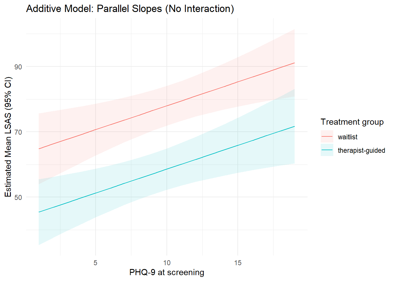

In the additive model, the lines are parallel: the difference between treatment groups is constant across PHQ-9.

8.2 Predicted means across PHQ-9 (interaction model)

plot_predictions(mod_lm_int, by = c("phq9_screen", "trt")) +
  labs(
    x = "PHQ-9 at screening",
    y = "Estimated Mean LSAS (95% CI)",
    color = "Treatment group",
    fill = "Treatment group",
    title = "Linear Interaction Model: Treatment Effect Varies with PHQ-9"
  ) +
  theme_minimal()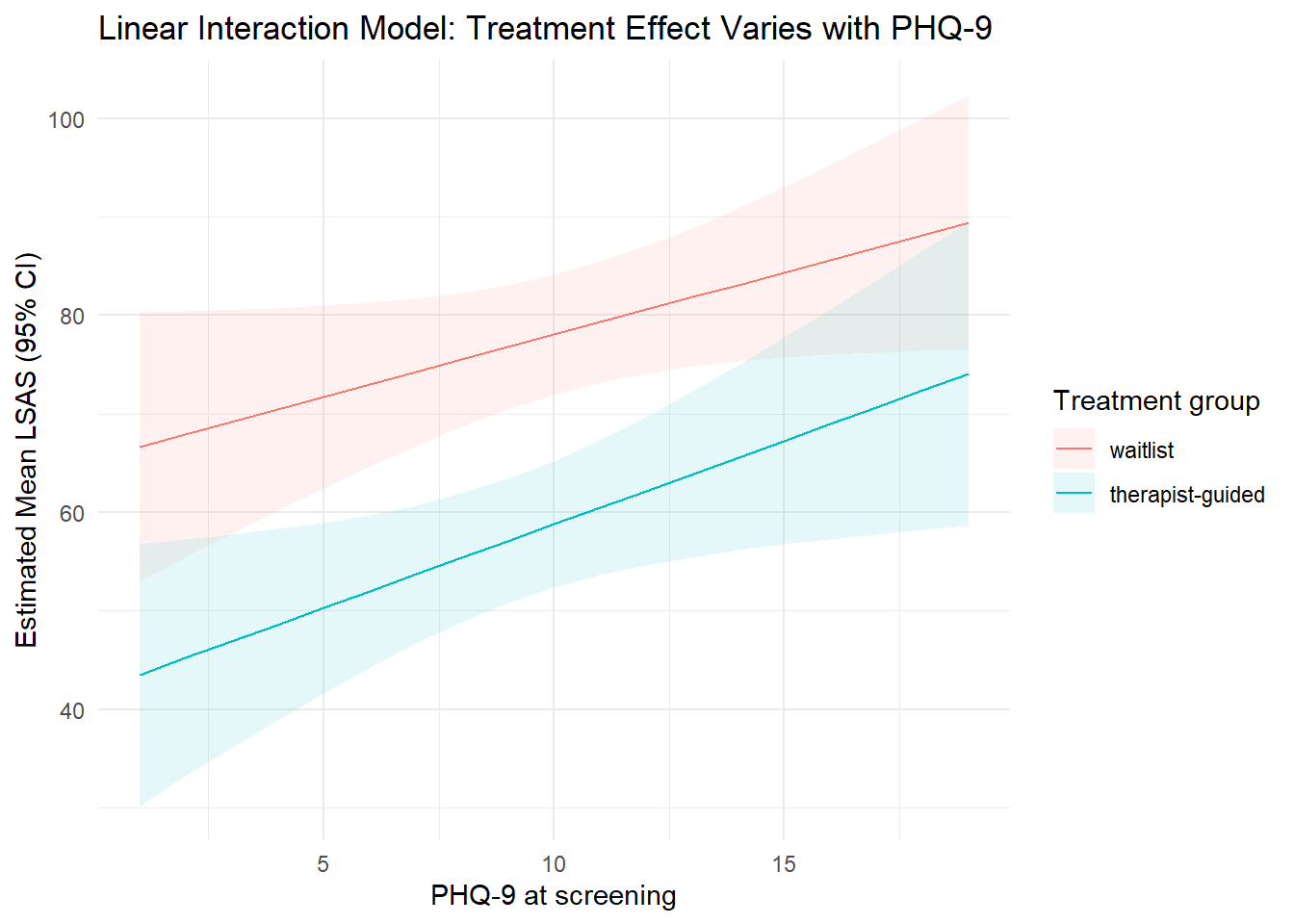

If the lines are not parallel, the treatment effect depends on baseline depression severity.

8.3 Visualizing the conditional treatment effect across PHQ-9

Instead of plotting predicted means, we can directly plot the estimated treatment effect as a function of PHQ-9, which makes it easier to gauge how much the treatment effect varies linearly with baseline PHQ-9 scores.

plot_comparisons(
  mod_lm_int,
  variables = "trt",
  by = "phq9_screen"
) +
  geom_hline(yintercept = 0, linetype = "dashed") +
  labs(
    x = "PHQ-9 at screening",
    y = "Estimated Treatment Effect (95% CI)",
    title = "Conditional Treatment Effect Across Baseline Depression"
  ) +
  theme_minimal()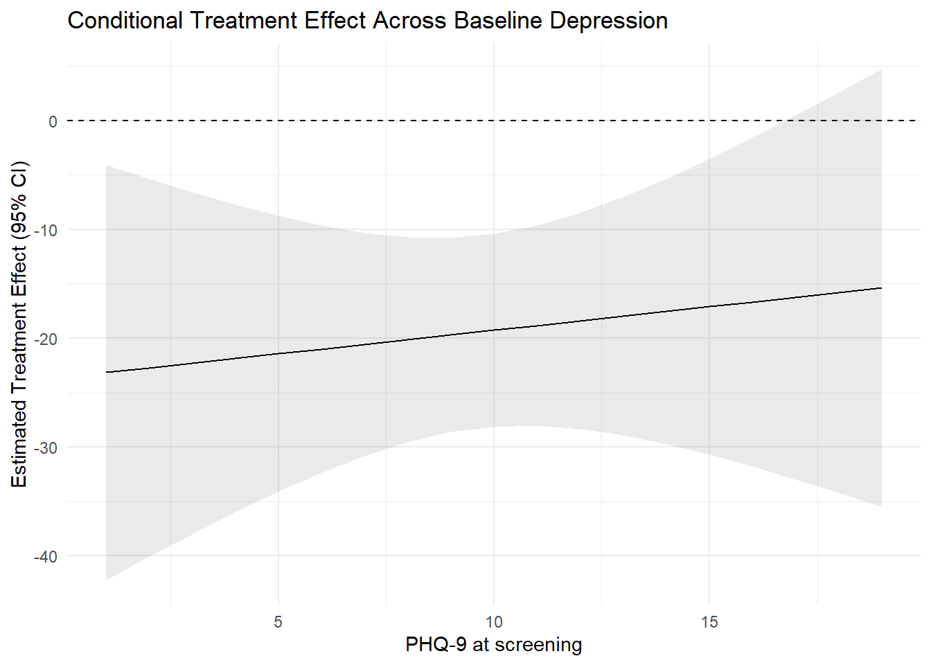

8.4 Non-linear interaction (Spline)

So far it does not seem like there is a substantial effect of baseline PHQ-9 scores on the treatment effect. However, it is possible that the effect varies non-linearly. We can investigate this by modeling PHQ-9 scores using a natural cubic spline.

library(splines)
library(patchwork)

# Fit spline regression
mod_lm_int_spline <- lm(
  lsas_post ~ trt * ns(phq9_screen, df = 4),
  data = df_red
)

# Plot predicted outcomes
p_spline_trend <- plot_predictions(
  mod_lm_int_spline,
  by = c("phq9_screen", "trt")
) +
  geom_rug(
    data = df_red,
    aes(x = phq9_screen, y = lsas_post),
    alpha = 0.25, position = "jitter", sides = "b"
  ) +
  geom_point(
    data = df_red,
    aes(phq9_screen, lsas_post, group = trt, color = trt),
    alpha = 0.5
  ) +
  labs(
    x = "PHQ-9 at screening",
    y = "Estimated Mean LSAS (95% CI)",
    color = "Treatment group",
    fill = "Treatment group",
    title = "Predicted Outcomes"
  ) +
  theme_minimal()

# Plot treatment effects
p_spline_es <- plot_comparisons(
  mod_lm_int_spline,
  variables = "trt",
  by = "phq9_screen"
) +
  geom_hline(yintercept = 0, linetype = "dashed") +
  labs(
    x = "PHQ-9 at screening",
    y = "Estimated Treatment Effect (95% CI)",
    color = "Treatment group",
    fill = "Treatment group",
    title = "Treatment Effect"
  ) +
  theme_minimal()

# Combine plots
(p_spline_trend + p_spline_es & theme(legend.position = "bottom")) +
  plot_layout(guides = "collect") +
  plot_annotation(
    title = paste(
      "Spline Interaction Model: Treatment Effect",
      "Varies Non-linearly with PHQ-9"
    )
  )

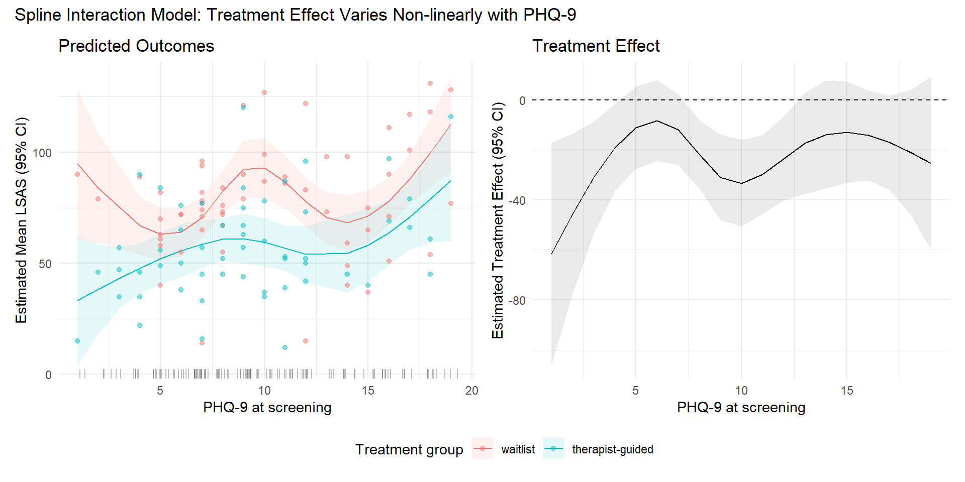
Caution

Do these curves make sense? Do we believe that the relationships are this wiggly? We should consider potential overfitting and fit a more constrained spline (e.g., changing df to 2 or 3)

8.5 Slightly More Complicated Hypothesis & Standardized Effects

We can estimate many other useful contrasts from the fitted model. For example, we might compare the treatment effect at PHQ-9 = 1 versus PHQ-9 = 15. The call below computes the difference between the two treatment effects at those PHQ-9 levels and then standardizes it by the baseline LSAS SD.

sd_baseline <- sd(df_red$lsas_screen, na.rm = TRUE)

avg_comparisons(
  mod_lm_int_spline,
  variables = "trt",
  by = "phq9_screen",
  newdata = datagrid(phq9_screen = c(1, 15)),
  hypothesis = ~ reference | contrast,
  transform = \(x) x / sd_baseline,
)

Hypothesis	Estimate	Pr(>\|z\|)	2.5 %	97.5 %
Type: response
(15) - (1)	2.7	0.06	-0.113	5.51

Interpretation

Estimated standardized difference in treatment effects between PHQ-9 = 1 and 15 is 2.7 SD units (95% CI: [-0.133, 5.51]).

Note: The order of values in newdata determines the direction of the contrast when using hypothesis = ~ reference | contrast (the result is contrast minus reference). Swap the order if you prefer the opposite difference.

We could also compare the treatment effect at each level of PHQ-9 screen to the mean of all effects

cmp_meandev <- avg_comparisons(
  mod_lm_int_spline,
  variables = "trt",
  by = "phq9_screen",
  transform = \(x) x / sd_baseline,
  hypothesis = ~ meandev | contrast
)
cmp_meandev

Hypothesis	Estimate	Pr(>\|z\|)	2.5 %	97.5 %
Type: response
(1) - Mean	-2.1030	0.0642	-4.3298	0.124
(2) - Mean	-1.2218	0.1177	-2.7522	0.309
(3) - Mean	-0.4127	0.4150	-1.4052	0.580
(4) - Mean	0.2518	0.5257	-0.5258	1.029
(5) - Mean	0.6995	0.1063	-0.1493	1.548
(6) - Mean	0.8582	0.0662	-0.0574	1.774
(7) - Mean	0.6557	0.1278	-0.1883	1.500
(8) - Mean	0.1087	0.7914	-0.6970	0.914
(9) - Mean	-0.4089	0.4013	-1.3636	0.546
(10) - Mean	-0.5393	0.2559	-1.4698	0.391
(11) - Mean	-0.3450	0.3905	-1.1324	0.442
(12) - Mean	0.0068	0.9870	-0.8116	0.825
(13) - Mean	0.3487	0.4958	-0.6546	1.352
(14) - Mean	0.5461	0.3170	-0.5234	1.616
(15) - Mean	0.5958	0.2276	-0.3721	1.564
(16) - Mean	0.5273	0.2014	-0.2816	1.336
(17) - Mean	0.3701	0.3926	-0.4783	1.219
(18) - Mean	0.1539	0.8073	-1.0826	1.390
(19) - Mean	-0.0919	0.9212	-1.9131	1.729

Let’s plot it and compare it to our previous treatment effect vs. PHQ-9 figure.

p_spline_meandev <- cmp_meandev |>
  mutate(phq9_screen = row_number() + 1) |>
  ggplot(aes(x = phq9_screen, y = estimate)) +
  geom_line() +
  geom_hline(yintercept = 0, linetype = "dashed") +
  geom_ribbon(aes(ymin = conf.low, ymax = conf.high), alpha = 0.15) +
  labs(
    title = "Deviations from Mean Effect",
    x = "PHQ-9 at screening",
    y = "Deviation from mean effect (SD units, 95% CI)"
  ) +
  theme_minimal()

p_spline_es + p_spline_meandev +
  plot_annotation(
    title = paste(
      "Spline Interaction Model: Treatment Effect",
      "Varies Non-linearly with PHQ-9"
    )
  )

Ignoring unknown labels:
• colour : "Treatment group"
• fill : "Treatment group"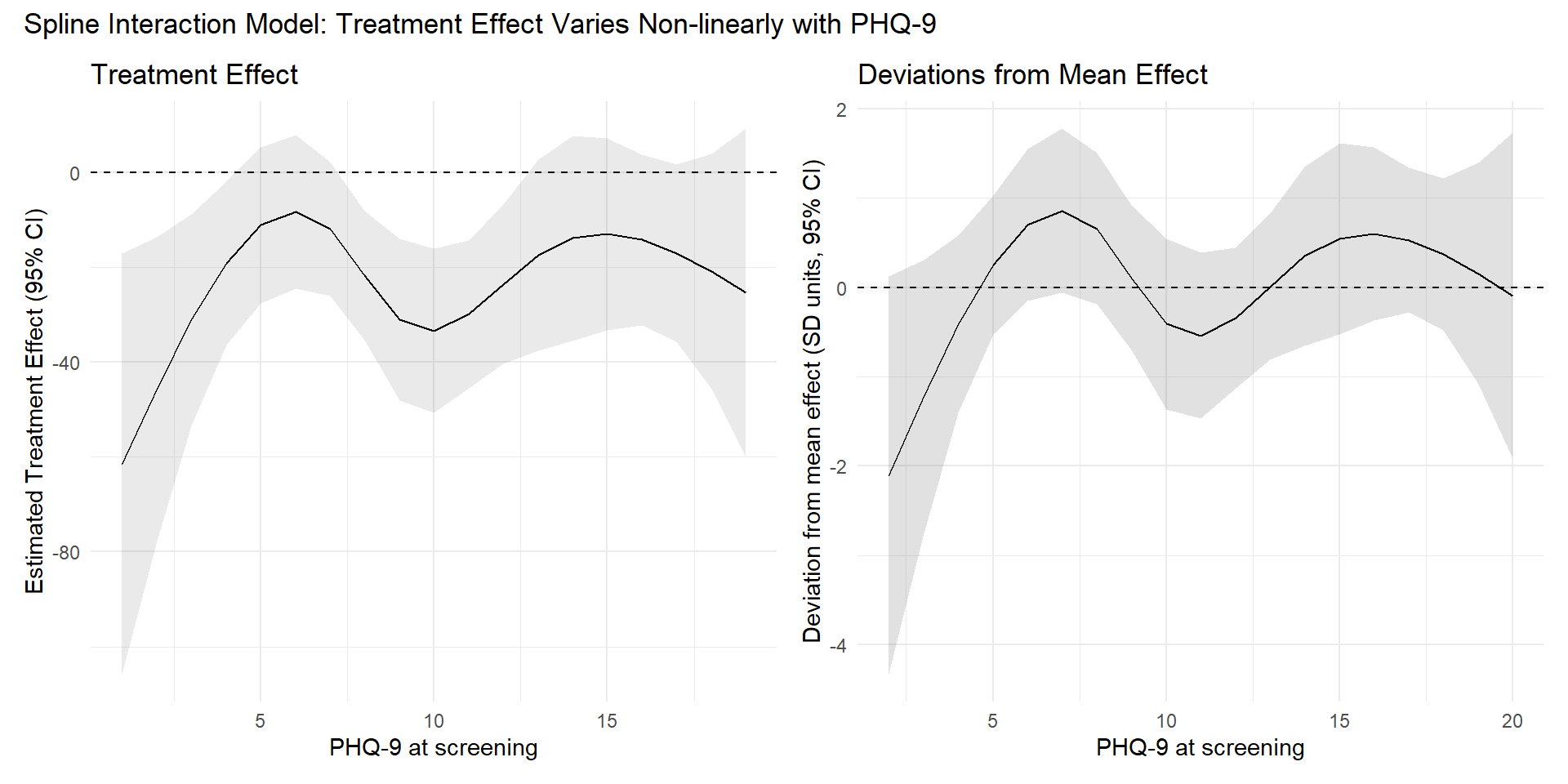

Note

The figure above illustrates point that the difference between “significant” and “not significant” is not itself statistically significant. In the left panel, the 95% CI for the treatment effect crosses 0 at some PHQ-9 values and not at others; this alone does not imply that the formal contrast between two treatment effects (e.g., PHQ-9 = 1 vs 15) is significant. The right panel shows that the direct comparison can be non-significant even when individual CIs differ in whether they include 0.

9 Summary

In this chapter you learned:

how to fit regression models with one binary and one numeric predictor
how conditional effects are interpreted when a moderator is continuous
the difference between additive (parallel slopes) and interaction models
how interactions change coefficient interpretation
how to estimate conditional and marginal effects using marginaleffects
how to visualize interactions using predicted values and treatment-effect curves

This chapter continues the foundation for working with multiple predictors, including both categorical and numeric variables.