1 Introduction

This chapter introduces the simplest possible regression model:
a model with no predictors, also known as an intercept-only model.

Even though the model is simple, it allows us to illustrate all core components of regression:

how R fits regression models
how to extract model estimates
how regression objects are structured
how to get model predictions using marginaleffects
how to visualize regression results
how to compute confidence intervals and standard errors

2 Packages and Functions

In this lab we use four core packages.

library(tidyverse) # Data wrangling and plotting
library(broom) # Converting model objects into tidy tables
library(quantreg) # Quantile regression (rq())
library(marginaleffects) # Predictions and uncertainty estimates
library(here)

Why these packages?

lm() fits linear regression models.
rq() fits quantile regression models.
broom helps inspect regression objects in tidy tables.
marginaleffects provides model-based predictions + standard errors + confidence intervals, even for quantile regression.
ggplot2 (part of tidyverse) allows flexible, reproducible visualizations.

2.1 Load the data

We’ll again use the dataset from the STePS study, which is an RCT comparing guided and unguided internet-delivered psychodynamic therapy for social anxiety disorder. The study is published online.

We assign this dataset to an object called df_clean.

df_clean <- read_csv2(here("data", "steps_clean.csv"))

3 Syntax of Intercept-Only Models in R

An intercept-only model estimates a single number:

the mean for linear regression
a quantile (e.g., median) for quantile regression

There are no predictors, so the model formula in R is simply:

lsas_post ~ 1

3.1 Formula for linear regression

In the context of linear regression, this is R syntax for the formula:

\[\mathbb{E}(LSAS_{post}) = \beta_0\]

Where $\mathbb{E}$ refers to the expected value (mean), and $\beta_0$ denotes the intercept. Sometimes, you may see this same model described using this formula:

\[LSAS_{post_i} = \beta_0 + \epsilon_i \]

That describes the same model, but highlights that the individual observations, denoted by $i$, are a function of the model intercept, $\beta_0$, and the error term, $_i $. The error term represents the unknown deviation of each observation from the population mean. Errors are closely related to residuals, which are the estimated errors calculated as the difference between observed values and fitted values.

3.2 Formula for Quantile Regression

Quantile regression allows us to model a chosen quantile of the outcome rather than the mean. For an intercept-only model estimating the $\tau$-th quantile, the corresponding formula is:

\[ Q_{LSAS\_{post}}(\tau) = \beta_{\tau} \]

Here, $Q_{LSAS\_{post}}(\tau)$ denotes the $\tau$-th quantile of the outcome. For example, if $\tau = 0.5$, the model estimates the median.

A parallel way to write this model, showing individual observations, denoted by $i$, is:

\[LSAS_{post_i} = \beta_{\tau} + e_i \]

This makes explicit that the “error term” $e_i$ is not assumed to have mean zero. Instead, it satisfies $P(e_i \le 0) = \tau$, meaning that:

when $\tau = 0.5$, half of the residuals fall below zero
when $\tau = 0.25$, 25% of residuals fall below zero
and so on

Thus, whereas linear regression models the mean, quantile regression models the chosen quantile of the outcome distribution, offering a more complete view when the distribution is skewed, heavy-tailed, or heterogeneous.

3.3 Linear regression (mean)

So let’s fit an intercept-only model for the score of the LSAS scale at post-treatment in the STePS study. First we use the lm() function to fit the regression model. To be able to easily access the model, we save it in an object called mod_lm. Using the summary() function on this regression object gives the most essential information about the model.

mod_lm <- lm(lsas_post ~ 1, data = df_clean)
summary(mod_lm)


Call:
lm(formula = lsas_post ~ 1, data = df_clean)

Residuals:
    Min      1Q  Median      3Q     Max 
-55.142 -18.142  -0.142  16.858  63.858 

Coefficients:
            Estimate Std. Error t value Pr(>|t|)    
(Intercept)   67.142      1.906   35.23   <2e-16 ***
---
Signif. codes:  0 '***' 0.001 '**' 0.01 '*' 0.05 '.' 0.1 ' ' 1

Residual standard error: 24.78 on 168 degrees of freedom
  (12 observations deleted due to missingness)

Here, the coefficient represents the estimated mean of the outcome. As this is an intercept-only model (i.e., no predictors), the estimated mean is identical to the sample mean:

mean(df_clean$lsas_post, na.rm = TRUE)

[1] 67.14201

3.4 Quantile regression (median)

Here we do the same thing as above, but use the rq() function to fit a quantile regression model, and the summary() function to get the most essential information.

mod_rq <- rq(lsas_post ~ 1, tau = 0.5, data = df_clean)
summary(mod_rq)


Call: rq(formula = lsas_post ~ 1, tau = 0.5, data = df_clean)

tau: [1] 0.5

Coefficients:
(Intercept) 
         67

The parameter tau sets the quantile:

tau = 0.5 → median
tau = 0.25 → 25th percentile
tau = 0.75 → 75th percentile

3.5 Quantile regression (25th percentile, median, 75th percentile)

We can also do the same for more than one quantile

mod_rq_ext <- rq(lsas_post ~ 1, tau = c(0.25, 0.5, 0.75), data = df_clean)
summary(mod_rq_ext)


Call: rq(formula = lsas_post ~ 1, tau = c(0.25, 0.5, 0.75), data = df_clean)

tau: [1] 0.25

Coefficients:
(Intercept) 
         49 

Call: rq(formula = lsas_post ~ 1, tau = c(0.25, 0.5, 0.75), data = df_clean)

tau: [1] 0.5

Coefficients:
(Intercept) 
         67 

Call: rq(formula = lsas_post ~ 1, tau = c(0.25, 0.5, 0.75), data = df_clean)

tau: [1] 0.75

Coefficients:
(Intercept) 
         84

The value of the intercept is the estimated quantile of the outcome. Again, since this is an intercept-only model, the value is the same as these quantiles in the sample.

quantile(df_clean$lsas_post, na.rm = TRUE)

  0%  25%  50%  75% 100% 
  12   49   67   84  131

4 Parts of the Regression Object

Model objects contain all components needed for inference. While the summary() function gives an overall summary of the model, there are several other functions to retrieve specific information from the regression objects.

4.1 Components of the linear model

You can use different functions to access information from the regression R object.

names(mod_lm) # gives the names of the different parts of the regression object

 [1] "coefficients"  "residuals"     "effects"       "rank"         
 [5] "fitted.values" "assign"        "qr"            "df.residual"  
 [9] "na.action"     "call"          "terms"         "model"

coef(mod_lm) # returns the coefficients from the object

(Intercept) 
   67.14201

head(fitted(mod_lm)) # gets the predicted values for each individual

       1        3        4        6        7        8 
67.14201 67.14201 67.14201 67.14201 67.14201 67.14201

head(residuals(mod_lm)) # returns the residuals

         1          3          4          6          7          8 
-17.142012   9.857988 -45.142012 -15.142012   7.857988 -22.142012

Key parts:

coefficients: the estimated mean
fitted values: all equal to the estimated mean in the intercept-only model
residuals: deviation of each observation from the fitted value (i.e. value predicted by the model)

You can also access specific information from the regression object by using the $ operator.

# the coefficients of the model (right now only the intercept)
mod_lm$coefficients

(Intercept) 
   67.14201

head(mod_lm$residuals) # the residuals (observed value - predicted value)

         1          3          4          6          7          8 
-17.142012   9.857988 -45.142012 -15.142012   7.857988 -22.142012

4.2 Components of the quantile regression model

names(mod_rq)

 [1] "coefficients"  "x"             "y"             "residuals"    
 [5] "dual"          "fitted.values" "na.action"     "formula"      
 [9] "terms"         "call"          "tau"           "rho"          
[13] "method"        "model"

coef(mod_rq)

(Intercept) 
         67

Quantile regression objects have similar structure, but contain quantile-specific information.

Again you can get information directly from the regression R object:

mod_rq$coefficients # the coefficient

(Intercept) 
         67

head(mod_rq$residuals) # the residuals (observed value - predicted value)

  1   3   4   6   7   8 
-17  10 -45 -15   8 -22

head(df_clean$lsas_post)

[1] 50 NA 77 22 NA 52

5 Getting Estimates Using `marginaleffects`

The marginaleffects package lets us extract:

predicted values
standard errors
confidence intervals

For intercept-only models, predictions are constant. As we have no predictors that can vary between subjects, predicted values are the same across all subjects.

5.1 Average prediction (linear regression)

avg_predictions(mod_lm)

Estimate	Std. Error	z	Pr(>\|z\|)	2.5 %	97.5 %
Type: response
67.1	1.91	35.2	<0.001	63.4	70.9

This returns:

estimated mean
standard error
confidence interval

5.2 Individual predictions

predictions(mod_lm) |> head()

Estimate	Std. Error	z	Pr(>\|z\|)	2.5 %	97.5 %
Type: response
67.1	1.91	35.2	<0.001	63.4	70.9
67.1	1.91	35.2	<0.001	63.4	70.9
67.1	1.91	35.2	<0.001	63.4	70.9
67.1	1.91	35.2	<0.001	63.4	70.9
67.1	1.91	35.2	<0.001	63.4	70.9
67.1	1.91	35.2	<0.001	63.4	70.9

These are equal for every observation because there are no predictors.

5.3 Median prediction (quantile regression)

avg_predictions(mod_rq)

Estimate	Std. Error	z	Pr(>\|z\|)	2.5 %	97.5 %
Type: response
67	2.52	26.6	<0.001	62.1	71.9

This returns the estimated median (or any other quantile selected).

6 Visualizing the Model with `ggplot2`

The visualization step shows how the estimated mean or median aligns with the empirical distribution.

6.1 Histogram with the estimated mean (linear model)

mean_est <- coef(mod_lm) # save the estimated mean from the linear model

# plot the mean over a histogram of the observed values
ggplot(df_clean, aes(lsas_post)) +
  geom_histogram(bins = 25, color = "white") +
  geom_vline(xintercept = mean_est, linewidth = 1.2) +
  labs(
    title = "Estimated Mean (Intercept-Only Linear Model)",
    x = "LSAS post-treatment score", y = "Frequency"
  ) +
  theme_minimal()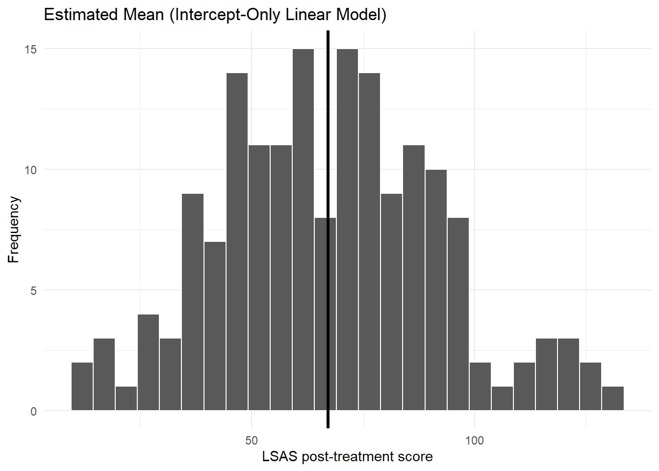

6.2 Estimated mean with confidence interval (linear model)

# get the estimated values from the linear regression model
ap <- avg_predictions(mod_lm)

# save as a tibble for plotting
df_plot <- tibble(
  mean_est = ap$estimate[1],
  lcl = ap$conf.low[1],
  ucl = ap$conf.high[1]
)

# use ggplot to create a plot
ggplot(df_plot, aes(y = 1, x = mean_est)) +
  geom_point(size = 3) +
  # add confidence interval
  geom_errorbar(aes(xmin = lcl, xmax = ucl), width = 0.1, linewidth = 1) +
  scale_y_continuous(breaks = NULL) + # remove the y-axis scale
  scale_x_continuous(limits = c(50, 90)) + # set x-axis range
  labs( # set labels
    y = "",
    x = "Estimated Mean (95% CI)"
  ) +
  theme_minimal()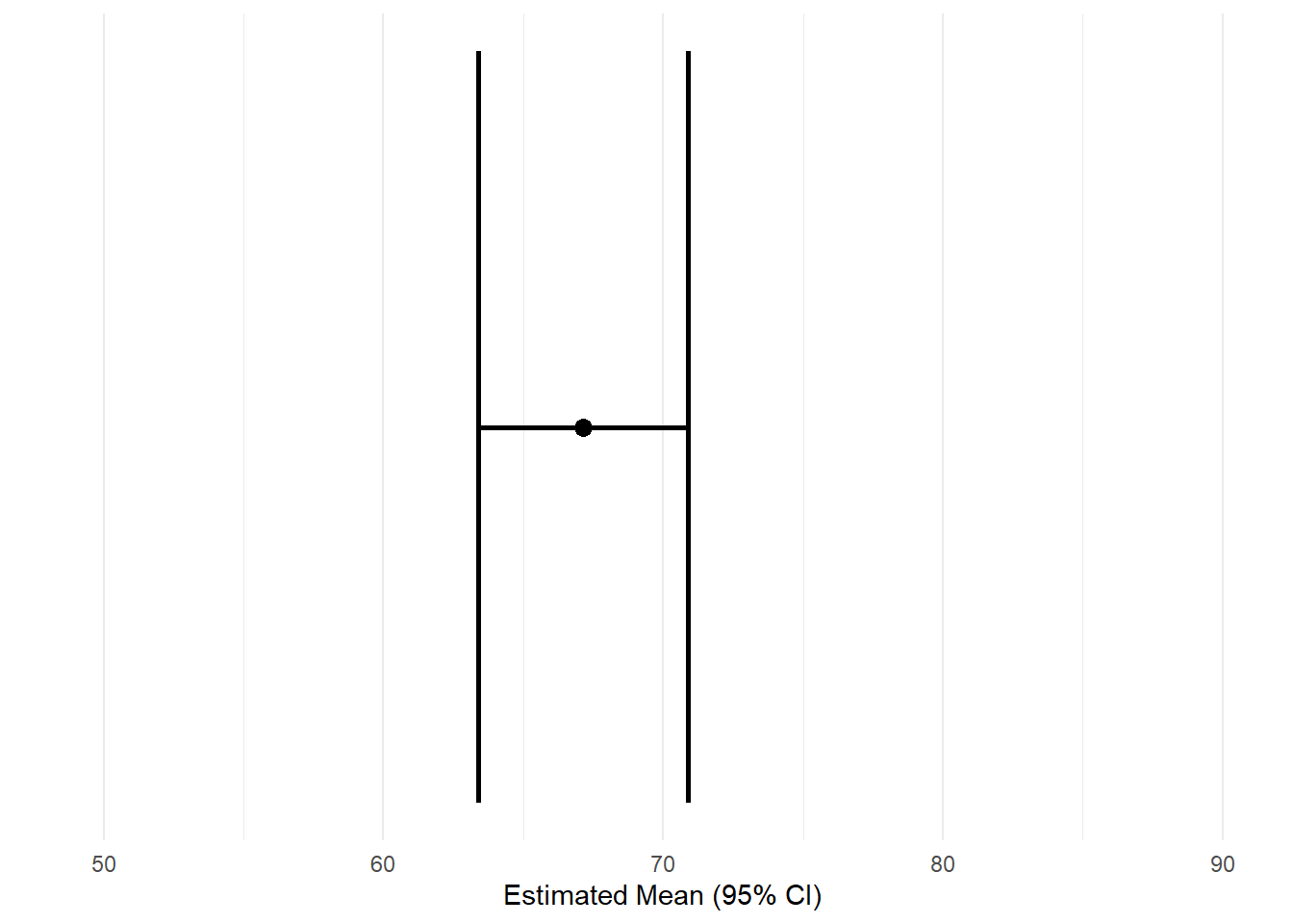

6.3 Histogram with median (quantile regression)

med_est <- coef(mod_rq)

ggplot(df_clean, aes(lsas_post)) +
  geom_histogram(bins = 25, color = "white") +
  geom_vline(xintercept = med_est, linewidth = 1.2) +
  labs(
    title = "Estimated Median (Intercept-Only Quantile Regression)",
    x = "LSAS post-treatment score", y = "Frequency"
  ) +
  theme_minimal()

Warning: Removed 12 rows containing non-finite outside the scale range
(`stat_bin()`).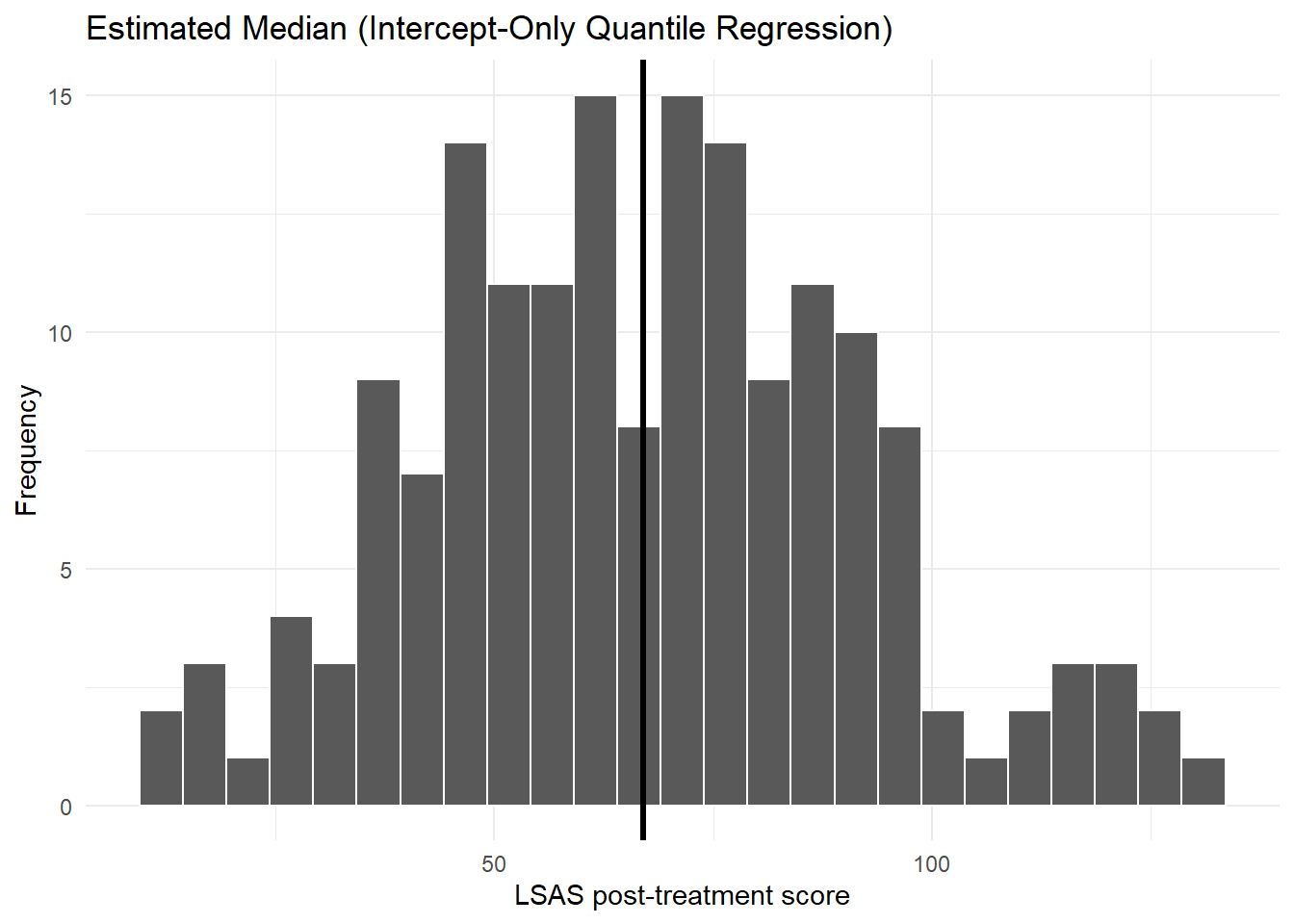

6.4 Estimated median with confidence interval (quantile regression)

# get the estimated values from the quantile regression model
ap <- avg_predictions(mod_rq)

# save as a tibble for plotting
df_plot <- tibble(
  med_est = ap$estimate[1],
  lcl = ap$conf.low[1],
  ucl = ap$conf.high[1]
)

# use ggplot to create a plot
ggplot(df_plot, aes(y = 1, x = med_est)) +
  geom_point(size = 3) +
  # add confidence interval
  geom_errorbar(aes(xmin = lcl, xmax = ucl), width = 0.1, linewidth = 1) +
  scale_y_continuous(breaks = NULL) + # remove the y-axis scale
  scale_x_continuous(limits = c(50, 90)) + # # set x-axis range
  labs( # set labels
    y = "",
    x = "Estimated Median (95% CI)"
  ) +
  theme_minimal()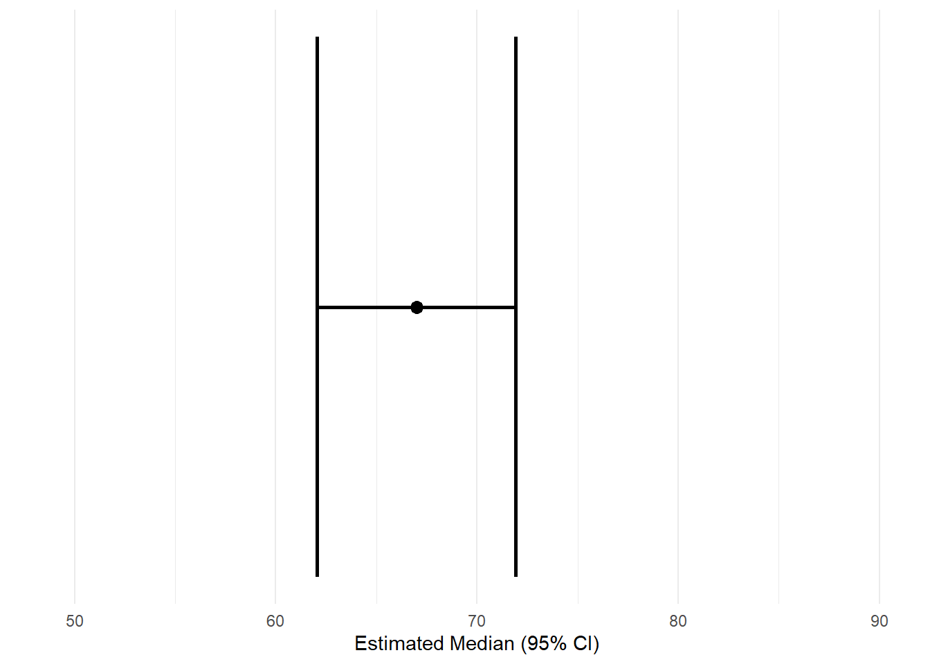

7 Confidence Intervals and Standard Errors

Regression models estimate a population quantity. As in the prior course, we need a measure of uncertainty.

7.1 Linear regression

R directly computes model-based CIs (which you can also get using the avg_predictions function):

confint(mod_lm)

               2.5 %   97.5 %
(Intercept) 63.37963 70.90439

For an intercept-only linear regression model, these confidence intervals are identical to the ones you would get from a one-sample t-test

t.test(df_clean$lsas_post)


    One Sample t-test

data:  df_clean$lsas_post
t = 35.231, df = 168, p-value < 2.2e-16
alternative hypothesis: true mean is not equal to 0
95 percent confidence interval:
 63.37963 70.90439
sample estimates:
mean of x 
 67.14201

7.2 Quantile regression

Quantile regression standard errors rely on resampling:

summary(mod_rq, se = "boot")


Call: rq(formula = lsas_post ~ 1, tau = 0.5, data = df_clean)

tau: [1] 0.5

Coefficients:
            Value    Std. Error t value  Pr(>|t|)
(Intercept) 67.00000  2.98941   22.41244  0.00000

Bootstrap SEs are often more stable for quantiles.

7.3 Using marginaleffects for CIs

7.3.1 Linear regression

avg_predictions(mod_lm, conf_level = 0.95)

Estimate	Std. Error	z	Pr(>\|z\|)	2.5 %	97.5 %
Type: response
67.1	1.91	35.2	<0.001	63.4	70.9

7.3.2 Quantile regression

avg_predictions(mod_rq, conf_level = 0.95)

Estimate	Std. Error	z	Pr(>\|z\|)	2.5 %	97.5 %
Type: response
67	2.52	26.6	<0.001	62.1	71.9

These produce:

estimate
standard error
lower confidence limit
upper confidence limit

All computed consistently across model types.

8 Summary

In this chapter you learned:

how to fit intercept-only regression models
the difference between linear (mean) and quantile (median) regression
the structure of model objects
how to extract prediction-based estimates using marginaleffects
how to visualize model summaries with ggplot
how to compute confidence intervals and standard errors

This chapter forms the foundation for working with models that include predictors, which we will explore in the next session.