1 Introduction

In the previous chapters, we studied regression models with:

a single binary predictor
a categorical predictor with multiple levels
a numeric predictor

In this chapter, we extend these ideas to two binary predictors.
This allows us to introduce the important concept of conditional effects and to distinguish between:

additive models (no interaction)
interaction models (effect modification)

You will learn:

how to interpret models with two binary predictors
what conditional effects mean
how interactions change interpretation
how to estimate and visualize effects using marginaleffects
how linear and quantile regression handle interactions

2 Packages and Data

library(tidyverse)
library(broom)
library(quantreg)
library(marginaleffects)
library(here)

2.1 Load data

df_clean <- read_csv2(here("data", "steps_clean.csv"))

One of the predictors will be treatment group. To get a binary variable (i.e., one with only two levels), we subset the data to include only participants in the therapist-guided or wait-list conditions. We’ll call this reduced dataset df_red.

df_red <- filter(df_clean, trt %in% c("therapist-guided", "waitlist"))

We convert trt to a factor and set waitlist as the reference group.

df_red <- df_red |>
  mutate(
    trt = factor(trt, levels = c("waitlist", "therapist-guided"))
  )

The other predictor will be depression severity. To get a binary variable, we dichotomize the PHQ-9 measure at screening using the sample median (for illustration only).

df_red <- df_red |>
  mutate(
    dep_bin = factor(
      phq9_screen > median(phq9_screen, na.rm = TRUE),
      levels = c(FALSE, TRUE),
      labels = c("Low", "High")
    )
  )

table(df_red$dep_bin) # show distribution


 Low High 
  65   55

3 Two Binary Predictors without Interaction (Additive Model)

We begin with a model that includes both predictors without an interaction.

3.1 Model formula

lsas_post ~ trt + dep_bin

lsas_post ~ trt + dep_bin

This corresponds to the linear regression model for the conditional mean:

\[ \begin{aligned} \mathbb{E}(LSAS_{post,i} \,\mid\, trt_i,\; dep\_bin_i) =& \beta_0 + \\ & \beta_1\, \mathbf{1}\{\text{trt}_i = \text{therapist-guided}\} + \\ & \beta_2\, \mathbf{1}\{\text{dep\_bin}_i = \text{High}\} \end{aligned} \]

Where:

\(\beta_0\): mean outcome in the reference group (waitlist & Low depression)
\(\beta_1\): conditional treatment effect, holding depression constant
\(\beta_2\): conditional depression effect, holding treatment constant

3.2 Interpretation of conditional effects

In this model:

the effect of treatment is assumed to be the same for low and high depression
the effect of depression is assumed to be the same in both treatment groups

This is called an additive model (because the effects of the two predictors are added to each other). Under additivity, the treatment effect is assumed the same in Low and High depression groups, and the depression effect is assumed the same in both treatment groups.

4 Linear Regression without Interaction

4.1 Fit the model

mod_lm_add <- lm(lsas_post ~ trt + dep_bin, data = df_red)
summary(mod_lm_add)


Call:
lm(formula = lsas_post ~ trt + dep_bin, data = df_red)

Residuals:
    Min      1Q  Median      3Q     Max 
-67.546 -14.212  -1.262  15.377  66.023 

Coefficients:
                    Estimate Std. Error t value Pr(>|t|)    
(Intercept)           74.623      3.870  19.281  < 2e-16 ***
trttherapist-guided  -20.646      4.576  -4.511 1.63e-05 ***
dep_binHigh            7.923      4.592   1.725   0.0873 .  
---
Signif. codes:  0 '***' 0.001 '**' 0.01 '*' 0.05 '.' 0.1 ' ' 1

Residual standard error: 24.16 on 109 degrees of freedom
  (8 observations deleted due to missingness)
Multiple R-squared:  0.1823,    Adjusted R-squared:  0.1673 
F-statistic: 12.15 on 2 and 109 DF,  p-value: 1.727e-05

4.1.1 Interpretation

Intercept: mean LSAS at post-treatment in waitlist & low depression.
trt coefficient: mean difference between therapist-guided and waitlist, adjusted for depression. The mean LSAS post score in the therapist-guided group is ~21 points lower than in the waitlist group.
dep_bin coefficient: mean difference between High and Low depression, adjusted for treatment. The mean LSAS post score in the Low-depression group is ~8 points lower than in the High-depression group.

4.2 Predicted means by group

We can now use the marginaleffects package to get the estimated means for each of the four groups, i.e., the conditional estimated means.

avg_predictions(mod_lm_add, by = c("trt", "dep_bin"))

trt	dep_bin	Estimate	Std. Error	z	Pr(>\|z\|)	2.5 %	97.5 %
Type: response
waitlist	Low	74.6	3.87	19.3	<0.001	67.0	82.2
waitlist	High	82.5	3.96	20.8	<0.001	74.8	90.3
therapist-guided	Low	54.0	3.83	14.1	<0.001	46.5	61.5
therapist-guided	High	61.9	4.21	14.7	<0.001	53.6	70.2

4.3 Treatment effect as a conditional contrast

We can get the conditional treatment effects across both groups using the marginaleffects package.

avg_comparisons(mod_lm_add,
  variables = "trt",
  by = "dep_bin"
)

dep_bin	Estimate	Std. Error	z	Pr(>\|z\|)	2.5 %	97.5 %
Type: response
Low	-20.6	4.58	-4.51	<0.001	-29.6	-11.7
High	-20.6	4.58	-4.51	<0.001	-29.6	-11.7

Since we specified the model as additive, the treatment effect is the same in both depression groups.

4.4 Treatment effect as a marginal contrast

The marginal contrast averages over the conditional contrasts. Since these are the same in this model, the marginal effect will be identical to the conditional effects.

avg_comparisons(mod_lm_add, variables = "trt")

Estimate	Std. Error	z	Pr(>\|z\|)	2.5 %	97.5 %
Type: response
-20.6	4.58	-4.51	<0.001	-29.6	-11.7

5 Adding an Interaction

Now we allow the treatment effect to differ depending on depression severity.

5.1 Model formula with interaction

lsas_post ~ trt * dep_bin

lsas_post ~ trt * dep_bin

Which expands, using indicator functions, to the conditional mean:

\[ \begin{aligned} \mathbb{E}(LSAS_{post,i} \,\mid\, trt_i,\; dep\_bin_i) =& \beta_0 + \\ & \beta_1\, \mathbf{1}\{\text{trt}_i = \text{therapist-guided}\} + \\ & \beta_2\, \mathbf{1}\{\text{dep\_bin}_i = \text{High}\} + \\ & \beta_3\, \mathbf{1}\{\text{trt}_i = \text{therapist-guided}\}\times \mathbf{1}\{\text{dep\_bin}_i = \text{High}\} \end{aligned} \]

\(\beta_3\) is the interaction term
it captures how the treatment effect changes with depression level

We now allow for different treatment effects depending on the level of depression, rather than the treatment effect simply adding to the depression effect as in the additive model.

6 Linear Regression with Interaction

6.1 Fit the interaction model

mod_lm_int <- lm(lsas_post ~ trt * dep_bin, data = df_red)
summary(mod_lm_int)


Call:
lm(formula = lsas_post ~ trt * dep_bin, data = df_red)

Residuals:
    Min      1Q  Median      3Q     Max 
-68.964 -13.517  -0.237  14.286  64.742 

Coefficients:
                                Estimate Std. Error t value Pr(>|t|)    
(Intercept)                       73.300      4.424  16.570  < 2e-16 ***
trttherapist-guided              -18.042      6.205  -2.907  0.00442 ** 
dep_binHigh                       10.664      6.367   1.675  0.09683 .  
trttherapist-guided:dep_binHigh   -5.748      9.220  -0.624  0.53427    
---
Signif. codes:  0 '***' 0.001 '**' 0.01 '*' 0.05 '.' 0.1 ' ' 1

Residual standard error: 24.23 on 108 degrees of freedom
  (8 observations deleted due to missingness)
Multiple R-squared:  0.1852,    Adjusted R-squared:  0.1626 
F-statistic: 8.183 on 3 and 108 DF,  p-value: 5.869e-05

6.1.1 Interpretation

The treatment effect is conditional on depression severity
Main effects are now interpreted at the reference level of the other variable
The interaction coefficient represents the difference in the treatment effect between participants with high versus low depression. It tells us that the treatment effect is ~6 points greater in the high-depression group compared with the treatment effect in the low-depression group.

6.2 Conditional treatment effects

avg_comparisons(
  mod_lm_int,
  variables = "trt",
  by = "dep_bin"
)

dep_bin	Estimate	Std. Error	z	Pr(>\|z\|)	2.5 %	97.5 %
Type: response
Low	-18.0	6.21	-2.91	0.00364	-30.2	-5.88
High	-23.8	6.82	-3.49	< 0.001	-37.2	-10.43

These estimates answer:

What is the treatment effect within each level of depression severity (low vs high)?

In this interaction model, the treatment effect is allowed to differ depending on baseline depression.

6.3 Marginal treatment effects

avg_comparisons(
  mod_lm_int,
  variables = "trt"
)

Estimate	Std. Error	z	Pr(>\|z\|)	2.5 %	97.5 %
Type: response
-20.7	4.59	-4.5	<0.001	-29.7	-11.7

This estimate is the marginal (population-average) treatment effect. It is obtained by averaging the conditional treatment effects over the observed distribution of low and high depression in the sample. Because we allowed the effect to differ between the depression groups, this estimate is no longer identical to the conditional estimate of trt from the model, or to the conditional contrasts above.

7 Quantile Regression with Two Binary Predictors

Now let’s do the same thing with quantile regression.

7.1 Additive model (median differences)

mod_rq_add <- rq(
  lsas_post ~ trt + dep_bin,
  tau = 0.5,
  data = df_red
)
summary(mod_rq_add)


Call: rq(formula = lsas_post ~ trt + dep_bin, tau = 0.5, data = df_red)

tau: [1] 0.5

Coefficients:
                    coefficients lower bd  upper bd 
(Intercept)          74.00000     61.64348  81.35652
trttherapist-guided -24.00000    -32.87924 -14.24152
dep_binHigh          10.00000     -4.86453  16.86453

7.2 Interaction model (median differences)

mod_rq_int <- rq(
  lsas_post ~ trt * dep_bin,
  tau = 0.5,
  data = df_red
)
summary(mod_rq_int)


Call: rq(formula = lsas_post ~ trt * dep_bin, tau = 0.5, data = df_red)

tau: [1] 0.5

Coefficients:
                                coefficients lower bd  upper bd 
(Intercept)                      74.00000     68.36922  78.54359
trttherapist-guided             -22.00000    -30.47806 -10.56581
dep_binHigh                      12.00000     -2.15693  20.25540
trttherapist-guided:dep_binHigh -11.00000    -22.36022  11.36022

7.3 Conditional median treatment effects

avg_comparisons(
  mod_rq_int,
  variables = "trt",
  by = "dep_bin"
)

dep_bin	Estimate	Std. Error	z	Pr(>\|z\|)	2.5 %	97.5 %
Type: response
Low	-22	5.60	-3.93	<0.001	-33.0	-11.0
High	-33	9.77	-3.38	<0.001	-52.2	-13.8

7.4 Marginal median treatment effects

avg_comparisons(
  mod_rq_int,
  variables = "trt"
)

Estimate	Std. Error	z	Pr(>\|z\|)	2.5 %	97.5 %
Type: response
-27	5.4	-5.01	<0.001	-37.6	-16.4

8 Visualization

8.1 Group means (additive vs interaction model)

p_add <- plot_predictions(
  mod_lm_add,
  by = c("trt", "dep_bin")
) +
  geom_line(
    aes(trt, estimate, group = dep_bin, color = dep_bin),
    position = position_dodge(0.1)
  ) +
  labs(
    x = "Treatment group",
    y = "Estimated Mean LSAS (95% CI)",
    color = "Depression",
    title = "Additive Model"
  ) +
  ylim(40, 95) +
  theme_minimal()

library(patchwork)
p_int <- plot_predictions(
  mod_lm_int,
  by = c("trt", "dep_bin")
) +
  geom_line(
    aes(trt, estimate, group = dep_bin, color = dep_bin),
    position = position_dodge(0.1)
  ) +
  labs(
    x = "Treatment group",
    y = "Estimated Mean LSAS (95% CI)",
    color = "Depression",
    title = "Interaction Model"
  ) +
  ylim(40, 95) +
  theme_minimal()

p_add + p_int + plot_layout(guides = "collect", axes = "collect")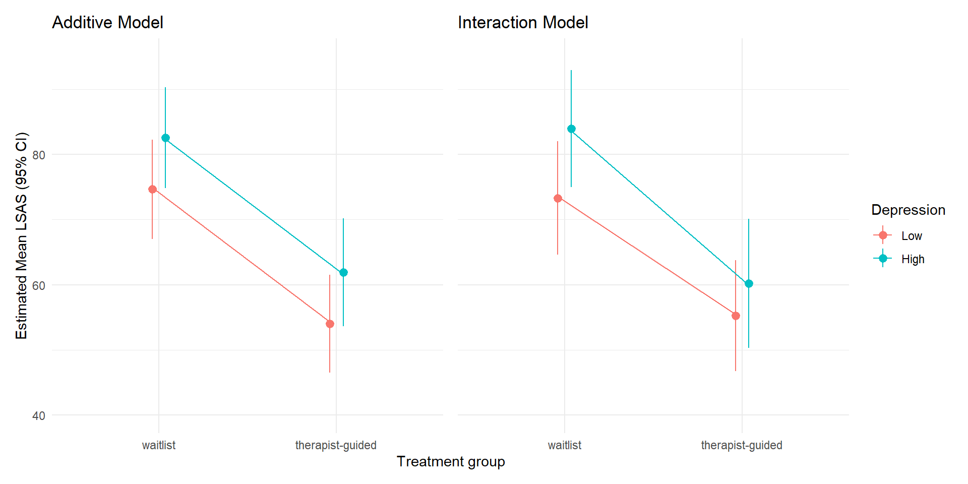

Here we see the difference between the additive and the interaction model clearly. Since the additive model assumed additivity, the lines are exactly parallel (i.e., the treatment effect is the same for the low vs high depression group). In the interaction model, we have allowed the treatment effects to differ by depression level, and we see that the high-depression group improves more than the low depression group.

9 Summary

In this chapter you learned:

how to fit regression models with two binary predictors
the meaning of conditional effects
the difference between additive and interaction models
how interactions change coefficient interpretation
how to estimate conditional effects using marginaleffects
how to visualize interactions using predicted values

This chapter completes the foundation for understanding effect modification, which is essential for applied regression and causal interpretation.