1 Introduction

In the previous chapter, we studied regression with a binary predictor.
In this chapter, we extend that framework to a categorical predictor with three levels, called trt.

This is a common situation in experiments with more than two arms (e.g., waitlist vs two treatment variants). The main difference compared to the binary case is that the model now estimates:

the expected outcome in a reference group
the difference between each other group and the reference group

You will learn:

how categorical predictors are represented using factors in R
how to interpret intercepts and coefficients with 3+ groups
how to obtain predicted values for each group
how to compute and visualize pairwise group differences
how linear (mean) and quantile (median) regression handle categorical predictors

2 Packages and Data

library(tidyverse)
library(broom)
library(quantreg)
library(marginaleffects)
library(here)

2.1 Load data

df_clean <- read_csv2(here("data", "steps_clean.csv"))

ℹ Using "','" as decimal and "'.'" as grouping mark. Use `read_delim()` for more control.

Rows: 181 Columns: 37
── Column specification ────────────────────────────────────────────────────────
Delimiter: ";"
chr  (1): trt
dbl (34): id, lsas_screen, gad_screen, phq9_screen, bbq_screen, scs_screen, ...
num  (2): dmrsodf_screen, dmrsodf_post

ℹ Use `spec()` to retrieve the full column specification for this data.
ℹ Specify the column types or set `show_col_types = FALSE` to quiet this message.

We will again use the treatment indicator variable trt as our predictor. In the original data, this indicator has three levels:

table(df_clean$trt)


     self-guided therapist-guided         waitlist 
              61               60               60

To make sure R treats trt as a categorical predictor, we convert it to a factor and choose a reference level.

As in the last chapter, we set waitlist as the reference group.

df_clean <- df_clean |>
  mutate(trt = factor(trt,
    levels = c("waitlist", "therapist-guided", "self-guided")
  ))
levels(df_clean$trt)

[1] "waitlist"         "therapist-guided" "self-guided"

Now we have the dummy coding:

contrasts(df_clean$trt)

                 therapist-guided self-guided
waitlist                        0           0
therapist-guided                1           0
self-guided                     0           1

3 Regression with a Categorical Predictor

With a categorical predictor with three levels, the regression model estimates:

the expected outcome in the reference group
the difference between each of the other groups and the reference group

3.1 Model formula

lsas_post ~ trt

The R syntax is the same as with the binary predictor. However, when trt has three levels, R uses dummy coding by default (also called treatment coding).

If waitlist is the reference group, the linear regression model can be written:

\[ \mathbb{E}(LSAS_{post} \mid trt) = \beta_0 + \beta_1 \, \mathbf{1}\{trt = \text{therapist-guided}\} + \beta_2 \, \mathbf{1}\{trt = \text{self-guided}\} \]

Where:

\(\beta_0\) is the expected outcome in the reference group (waitlist)
\(\beta_1\) is the mean difference between therapist-guided and waitlist
\(\beta_2\) is the mean difference between self-guided and waitlist
\(\mathbf{1}\{\cdot\}\) is the indicator function which is 1 if the condition holds and 0 otherwise

trt	Predicted value
waitlist	\(\beta_0\)
therapist-guided	\(\beta_0 + \beta_1\)
self-guided	\(\beta_0 + \beta_2\)

So the coefficients compare each treatment arm to the reference group.

4 Linear Regression (Mean Differences)

4.1 Fit the model

mod_lm <- lm(lsas_post ~ trt, data = df_clean)
summary(mod_lm)


Call:
lm(formula = lsas_post ~ trt, data = df_clean)

Residuals:
    Min      1Q  Median      3Q     Max 
-64.448 -14.912  -1.352  14.088  62.648 

Coefficients:
                    Estimate Std. Error t value Pr(>|t|)    
(Intercept)           78.448      3.062  25.623  < 2e-16 ***
trttherapist-guided  -21.096      4.409  -4.785 3.76e-06 ***
trtself-guided       -13.536      4.349  -3.113  0.00218 ** 
---
Signif. codes:  0 '***' 0.001 '**' 0.01 '*' 0.05 '.' 0.1 ' ' 1

Residual standard error: 23.32 on 166 degrees of freedom
  (12 observations deleted due to missingness)
Multiple R-squared:  0.1248,    Adjusted R-squared:  0.1143 
F-statistic: 11.84 on 2 and 166 DF,  p-value: 1.561e-05

Interpretation

(Intercept): wait-list mean
trttherapist-guided: mean difference for the therapist-guided vs wait-list
trtself-guided: mean difference for the self-guided group vs wait-list

We can verify group means directly:

df_clean |>
  group_by(trt) |>
  summarize(mean_lsas = mean(lsas_post, na.rm = TRUE))

trt	mean_lsas
waitlist	78.44828
therapist-guided	57.35185
self-guided	64.91228

4.2 Relationship to one-way ANOVA

A linear regression with one categorical predictor (3+ groups) is equivalent to a one-way ANOVA:

anova(mod_lm)

	Df	Sum Sq	Mean Sq	F value	Pr(>F)
trt	2	12873.37	6436.685	11.83959	1.56e-05
Residuals	166	90247.22	543.658	NA	NA

The ANOVA table tests whether there is evidence that at least one group mean differs.

5 Quantile Regression (Quantile Differences)

5.1 Model formulation

For quantile regression at quantile \(\tau\):

\[ Q_{LSAS_{post}}(\tau) = \beta_0(\tau) + \beta_1(\tau) \, \mathbf{1}\{trt = \text{therapist-guided}\} + \beta_2(\tau) \, \mathbf{1}\{trt = \text{self-guided}\} \]

\(\beta_0(\tau)\) = \(\tau\)-th quantile in waitlist
\(\beta_1(\tau)\) = \(\tau\)-th quantile difference (therapist-guided − waitlist)
\(\beta_2(\tau)\) = \(\tau\)-th quantile difference (self-guided − waitlist)

5.2 Fit a median regression

mod_rq <- rq(lsas_post ~ trt, tau = 0.5, data = df_clean)
summary(mod_rq)


Call: rq(formula = lsas_post ~ trt, tau = 0.5, data = df_clean)

tau: [1] 0.5

Coefficients:
                    coefficients lower bd  upper bd 
(Intercept)          77.00000     71.70143  84.59713
trttherapist-guided -24.00000    -31.74701 -16.62650
trtself-guided      -13.00000    -18.30306  -2.13129

Again, the interpretation of the coefficients is the same as in linear regression, but now refers to quantiles.

Verify group medians directly:

df_clean |>
  group_by(trt) |>
  summarize(median_lsas = median(lsas_post, na.rm = TRUE))

trt	median_lsas
waitlist	77.0
therapist-guided	52.5
self-guided	64.0

6 Predictions Using `marginaleffects`

As in the binary predictor case, marginaleffects makes it easy to get:

predicted values for each group
uncertainty (SEs and CIs)
group differences as contrasts

6.1 Predicted means by group (linear regression)

avg_predictions(mod_lm, by = "trt")

trt	Estimate	Std. Error	z	Pr(>\|z\|)	2.5 %	97.5 %
Type: response
waitlist	78.4	3.06	25.6	<0.001	72.4	84.4
therapist-guided	57.4	3.17	18.1	<0.001	51.1	63.6
self-guided	64.9	3.09	21.0	<0.001	58.9	71.0

6.2 Predicted medians by group (quantile regression)

avg_predictions(mod_rq, by = "trt")

trt	Estimate	Std. Error	z	Pr(>\|z\|)	2.5 %	97.5 %
Type: response
waitlist	77	3.36	22.9	<0.001	70.4	83.6
therapist-guided	53	4.07	13.0	<0.001	45.0	61.0
self-guided	64	3.96	16.2	<0.001	56.2	71.8

6.3 Group differences as contrasts

6.3.1 Mean differences (linear regression)

With three groups, there is no single “treatment − control” difference. Instead, we usually calculate the pairwise mean differences between all groups.

cmp <- avg_comparisons(mod_lm, variables = list("trt" = "pairwise"))
cmp

Contrast	Estimate	Std. Error	z	Pr(>\|z\|)	2.5 %	97.5 %
Type: response
self-guided - therapist-guided	7.56	4.43	1.71	0.08773	-1.12	16.24
self-guided - waitlist	-13.54	4.35	-3.11	0.00185	-22.06	-5.01
therapist-guided - waitlist	-21.10	4.41	-4.78	< 0.001	-29.74	-12.45

6.3.2 Median differences (quantile regression)

cmp_med <- avg_comparisons(mod_rq, variables = list("trt" = "pairwise"))
cmp_med

Contrast	Estimate	Std. Error	z	Pr(>\|z\|)	2.5 %	97.5 %
Type: response
self-guided - therapist-guided	11	5.67	1.94	0.0525	-0.12	22.12
self-guided - waitlist	-13	5.19	-2.50	0.0123	-23.18	-2.82
therapist-guided - waitlist	-24	5.28	-4.55	<0.001	-34.34	-13.66

7 Visualization

7.1 Group means with confidence intervals

plot_predictions(mod_lm, by = "trt") +
  labs(
    x = "Treatment group",
    y = "Estimated Mean LSAS (95% CI)",
    title = "Estimated Group Means from Linear Regression"
  ) +
  theme_minimal()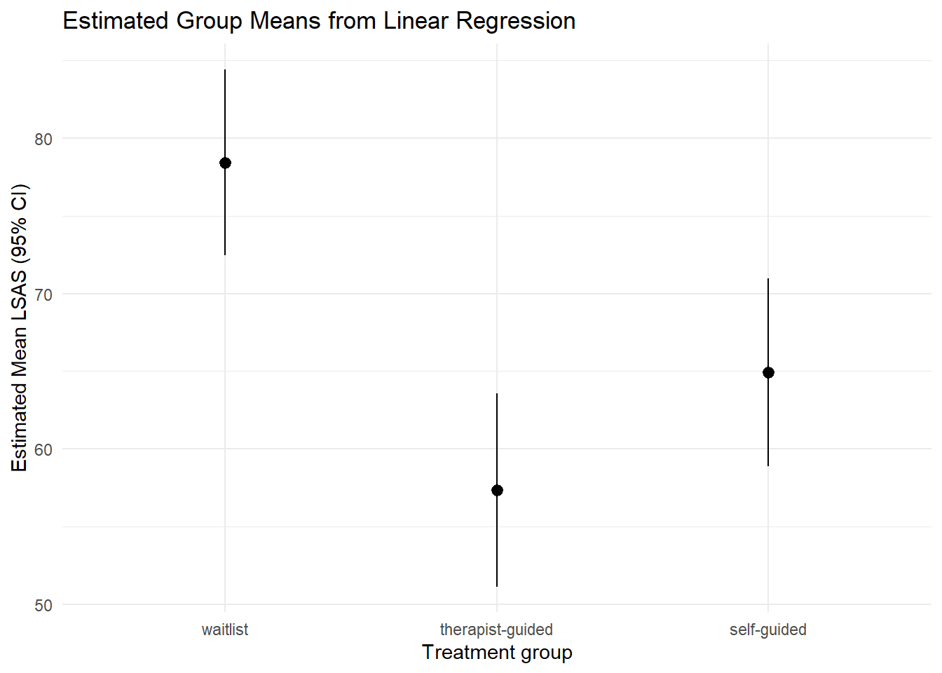

7.2 Group medians with confidence intervals

plot_predictions(mod_rq, by = "trt") +
  labs(
    x = "Treatment group",
    y = "Estimated Median LSAS (95% CI)",
    title = "Estimated Group Medians from Quantile Regression"
  ) +
  theme_minimal()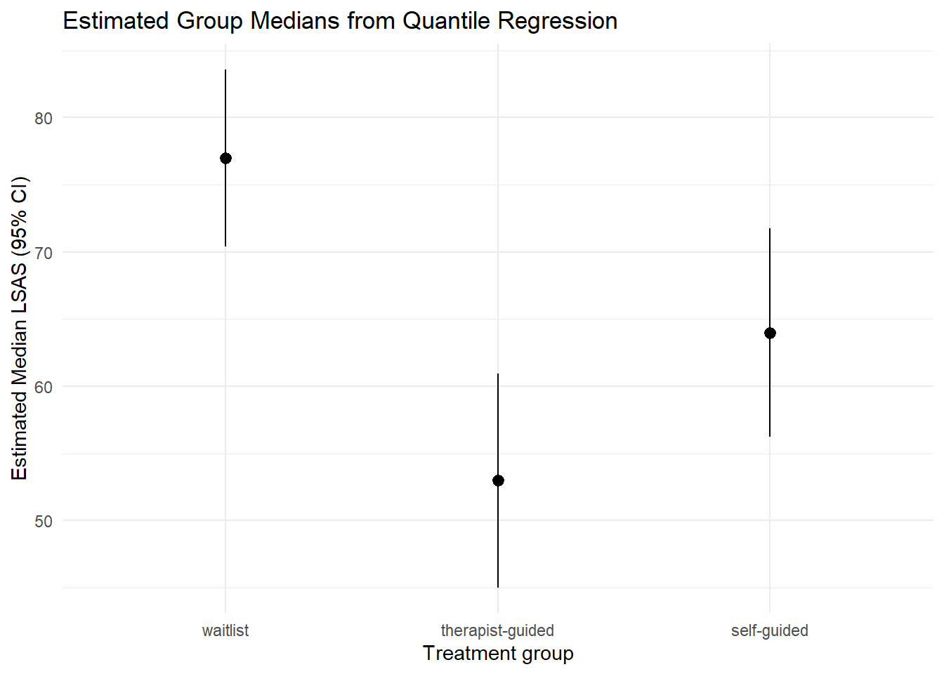

7.3 Mean differences (pairwise) with confidence intervals

cmp |>
  ggplot(aes(y = contrast, x = estimate)) +
  geom_vline(xintercept = 0, linetype = "dashed") +
  geom_point(size = 3) +
  geom_errorbar(aes(xmin = conf.low, xmax = conf.high), width = 0.1) +
  labs(
    y = "",
    x = "Estimated Mean Difference (95% CI)",
    title = "Pairwise Mean Differences (Linear Regression)"
  ) +
  theme_minimal()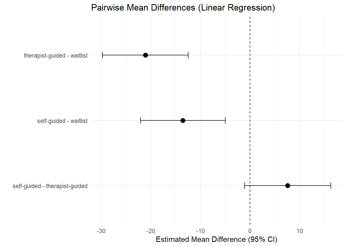

7.4 Median differences (pairwise) with confidence intervals

ggplot(cmp_med, aes(y = contrast, x = estimate)) +
  geom_vline(xintercept = 0, linetype = "dashed") +
  geom_point(size = 3) +
  geom_errorbar(aes(xmin = conf.low, xmax = conf.high), width = 0.1) +
  labs(
    y = "",
    x = "Estimated Median Difference (95% CI)",
    title = "Pairwise Median Differences (Quantile Regression)"
  ) +
  theme_minimal()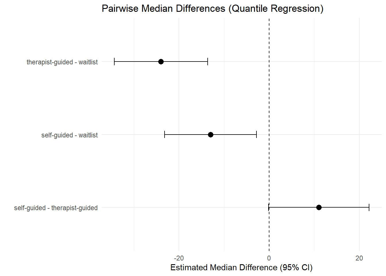

7.5 Ratio of Means and Other Hypotheses

As before, we can answer a range of other hypotheses. For example, the ratio of group outcomes.

avg_comparisons(
  mod_lm,
  variables = list("trt" = "pairwise"),
  comparison = "ratio"
)

Contrast	Estimate	Std. Error	z	Pr(>\|z\|)	2.5 %	97.5 %
Type: response
mean(self-guided) / mean(therapist-guided)	1.132	0.0826	13.7	<0.001	0.970	1.294
mean(self-guided) / mean(waitlist)	0.827	0.0509	16.3	<0.001	0.728	0.927
mean(therapist-guided) / mean(waitlist)	0.731	0.0495	14.8	<0.001	0.634	0.828

We could also compare each treatment group to the grand mean, instead of contrasting them with a reference group (the waitlist).

avg_predictions(
  mod_lm,
  by = "trt",
  hypothesis = ~meandev
)

Hypothesis	Estimate	Std. Error	z	Pr(>\|z\|)	2.5 %	97.5 %
Type: response
(waitlist) - Mean	11.54	2.52	4.583	<0.001	6.61	16.48
(therapist-guided) - Mean	-9.55	2.56	-3.725	<0.001	-14.58	-4.53
(self-guided) - Mean	-1.99	2.53	-0.787	0.431	-6.95	2.97

8 Summary

In this chapter you learned:

how to fit regression models with a categorical predictor (3 levels)
how dummy coding works (reference group + differences)
how linear regression estimates mean differences across groups
how quantile regression estimates quantile differences across groups
how to extract predicted values and contrasts using marginaleffects
how to visualize group means/medians and pairwise differences with confidence intervals