library(tidyverse)
library(here)
library(parameters)
library(splines)
library(performance)Chapter 7: Model Assumptions and Diagnostics
Introduction
In the previous chapters, we studied regression models with various types of predictors.
In this chapter, we focus on the key assumptions behind the linear regression model and practical ways to diagnose them in R.
You will learn the assumptions that most matter in practice:
- Linearity / correct specification
- Independent errors
- Constant error variance (homoscedasticity)
- Normality of errors (usually less critical for large sample sizes)
We use the performance package to quickly diagnose issues and show simple remedies. See the check_model vignette for details on the plots.
Packages and Data
Load Data
df_clean <- read_csv2(here("data", "steps_clean.csv"))STePS Model
Let’s perform a quick diagnostic of the ANCOVA‑style STePS model.
mod_lm <- lm(
  lsas_post ~ trt + lsas_screen + phq9_screen + gad_screen,
  data = df_clean
)
check_model(mod_lm)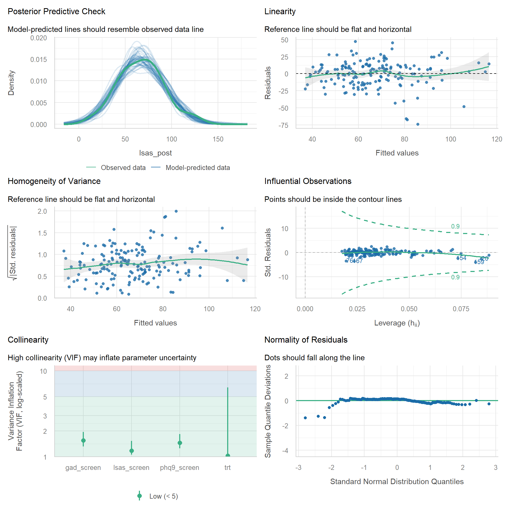
There are some possible problematic residual values in the left tail: a few participants report much lower observed values than predicted by the model. This is likely not a substantive issue.
Using Fake-Data Simulation to Understand Assumptions
Simulating data is a great way to understand model assumptions.
A Well-Behaved Base Model
n <- 180
x <- rnorm(n, 0, 1)
epsilon <- rnorm(n, 0, 1)
y <- 1 + 2 * x + epsilon

m_base <- lm(y ~ x)

check_model(m_base)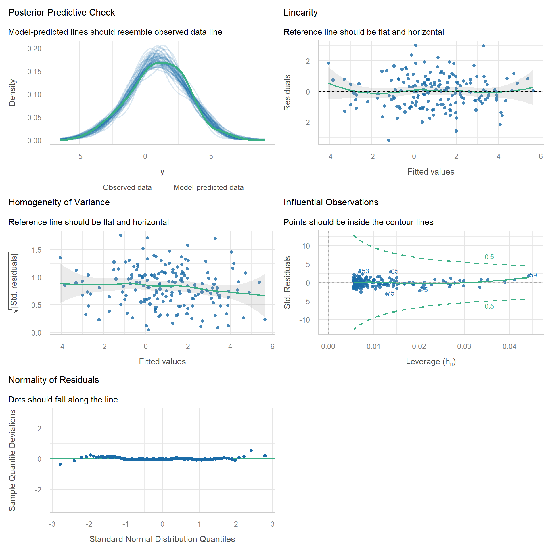
Note that even data simulated from a correctly specified regression model will deviate from perfection due to sampling variability.
Nonlinear Model
Now let’s break the linearity assumption by simulating from a quadratic function.
n <- 1000
x <- runif(n, -3, 3)
epsilon <- rnorm(n, 0, 2)
# linear slope = 0
y_nl <- 10 + 3 * x^2 + epsilon

# Wrong model spec
m_lin <- lm(y_nl ~ x)
check_model(m_lin)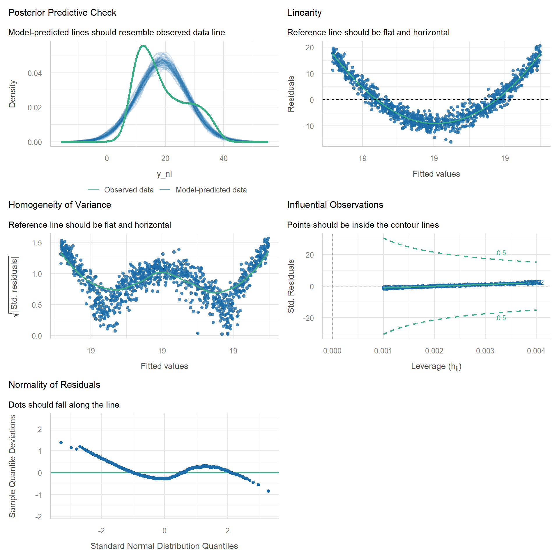
We can see that there are many issues with the model.
Fix 1: Add Polynomial Term
If we add a quadratic term then most issues should disappear.
m_quad <- lm(y_nl ~ x + I(x^2))
check_model(m_quad)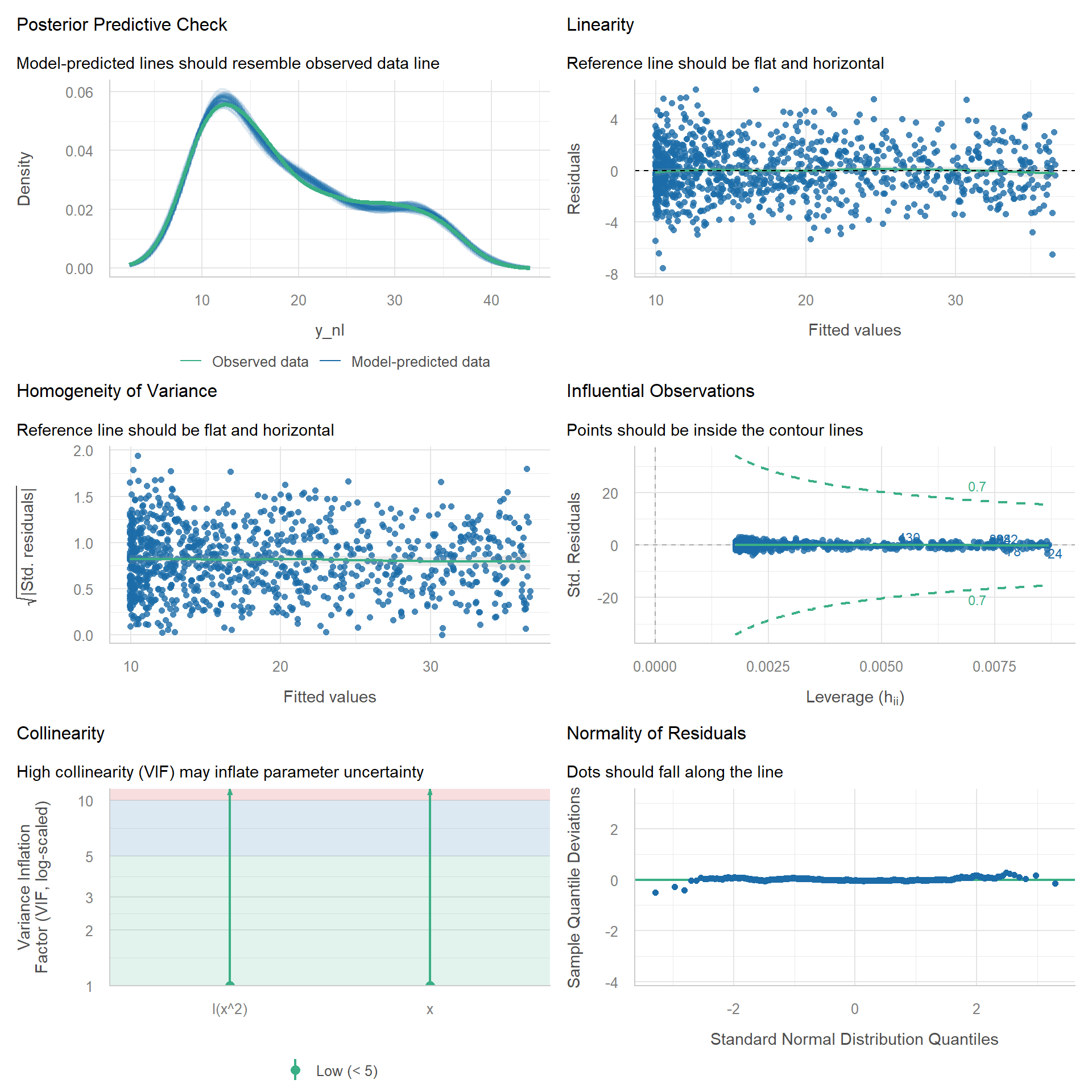
Fix 2: Natural Cubic Spline
As an illustration, a more flexible cubic spline should also remedy the problems.
m_spline <- lm(y_nl ~ ns(x, df = 4))
check_model(m_spline)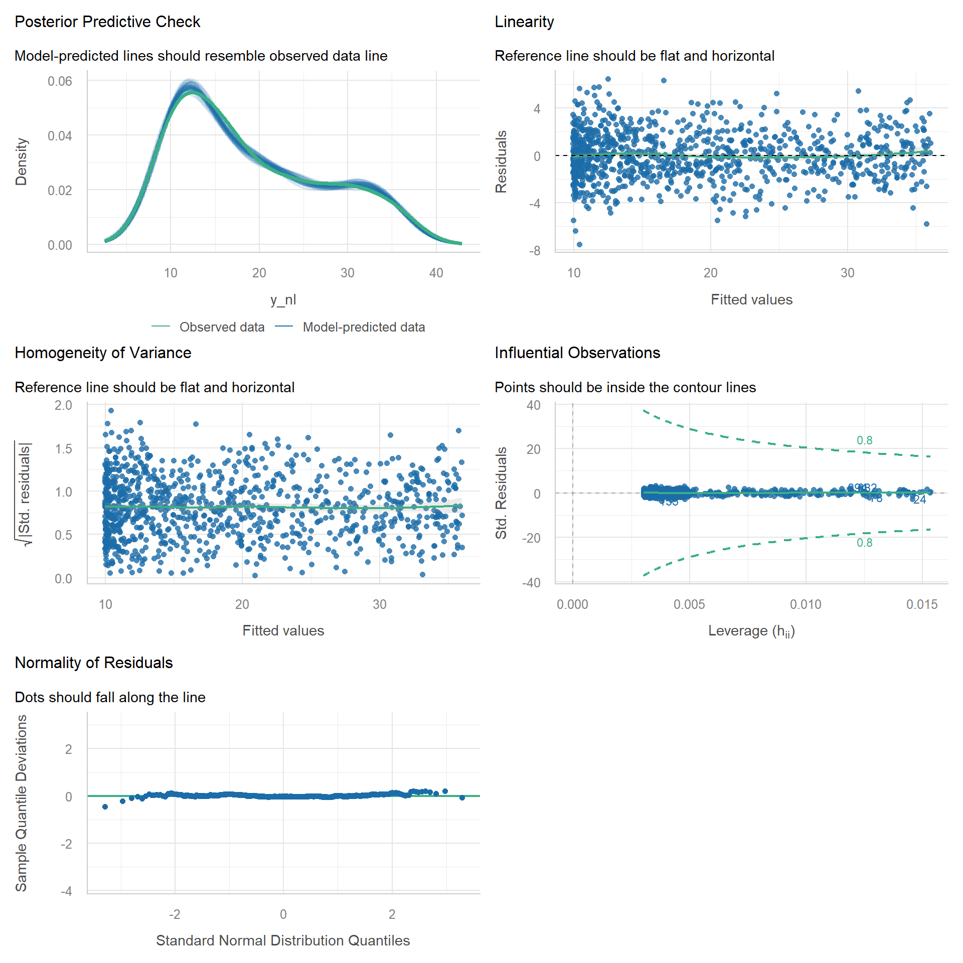
Let’s plot all the fits.
# Compare curves
nd <- data.frame(x = seq(min(x), max(x), length.out = 200))
nd$y_lin <- predict(m_lin, newdata = nd)
nd$y_quad <- predict(m_quad, newdata = nd)
nd$y_spline <- predict(m_spline, newdata = nd)

# Plot
p <- ggplot(data.frame(x = x, y = y_nl), aes(x, y)) +
  geom_point(alpha = 0.3, shape = 16) +
  geom_line(
    data = nd,
    aes(x, y = y_lin, color = "Linear (mis-specified)"),
    linewidth = 1
  ) +
  geom_line(
    data = nd,
    aes(x, y = y_quad, color = "Quadratic"),
    linewidth = 1
  ) +
  geom_line(
    data = nd,
    aes(x, y = y_spline, color = "Spline"),
    linewidth = 1
  ) +
  labs(
    title = "Nonlinearity: Linear vs Quadratic vs Spline",
    x = "x", y = "y", color = "Fit"
  ) +
  theme_minimal()

p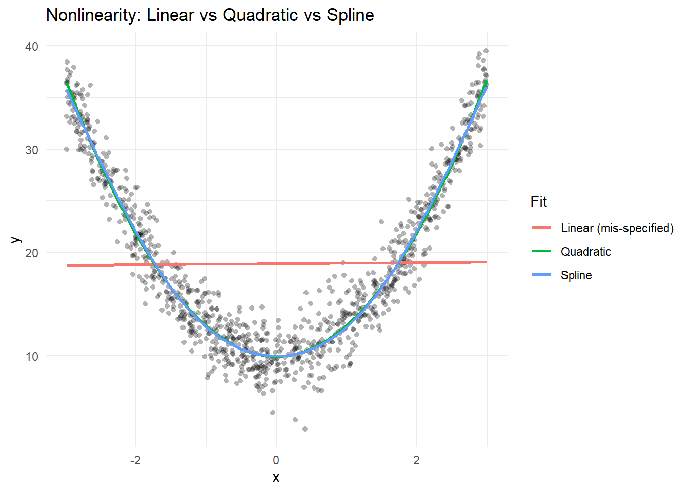
Clearly, the linear coefficient is not a good summary of the relationship.
Heteroskedasticity (Non-Constant Variance)
Let’s break the OLS assumptions by simulating data from a lognormal model, which will lead to heteroskedastic errors.
# Generate data from a lognormal distribution
gen_lnorm <- function(n) {
  x <- rnorm(n, 0, 1)
  mu <- 1 + 2 * x
  sdlog <- 0.5
  u <- rlnorm(n, meanlog = -sdlog^2 / 2, sdlog = sdlog) # so that E[u]=1
  y_lnorm <- mu * u

  data.frame(y = y_lnorm, x = x)
}
d_lnorm <- gen_lnorm(n = 300)
m_het <- lm(y ~ x, d_lnorm)
check_model(m_het)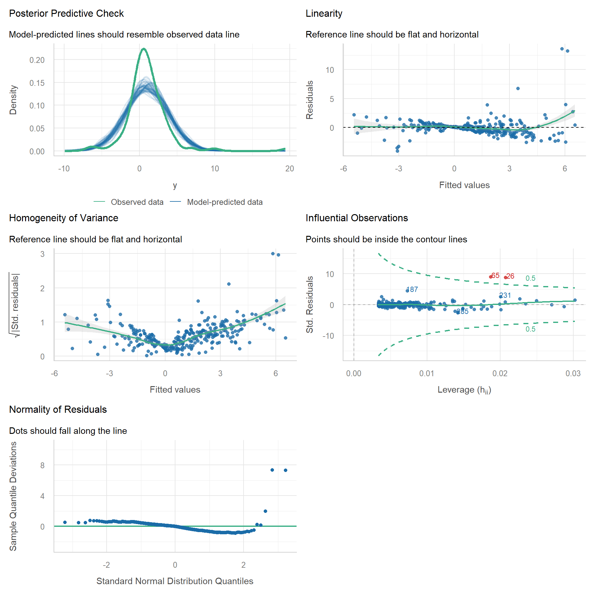
check_heteroscedasticity(m_het)Warning: Heteroscedasticity (non-constant error variance) detected (p < .001).We can see a clear deviation from constant variance. One remedy is to use robust standard errors.
compare_parameters(
  "standard" = model_parameters(m_het),
  "Robust SEs" = model_parameters(m_het, vcov = "HC3")
) |>
display()| Parameter | standard | Robust SEs |
|---|---|---|
| (Intercept) | 1.04 (0.87, 1.21) | 1.04 (0.86, 1.22) |
| x | 2.31 (2.13, 2.49) | 2.31 (1.97, 2.65) |
| Observations | 300 | 300 |
If we repeat this process, we can demonstrate that while the regression coefficient is correct, the standard error is wrong and therefore so are p-values and confidence intervals.
Code
# Helper functions for the simulation
library(mirai)
daemons(8)
set.seed(44334234)
everywhere({
  library(tidyverse)
  library(parameters)
})
run_sim <- function(
    data_gen_func,
    data_gen_params = list(NULL),
    formula,
    vcov = NULL,
    n_simulations = 1000) {
  map(
    seq_len(n_simulations),
    in_parallel( # nolint: object_usage_linter
      \(i) {
        d <- do.call(data_gen_func, data_gen_params)
        mod <- lm(formula, data = d)
        model_parameters(mod, vcov = vcov) |> as_tibble()
      },
      formula = formula,
      vcov = vcov,
      data_gen_func = data_gen_func,
      data_gen_params = data_gen_params
    )
  ) |>
    list_rbind()
}
summarize_sim <- function(x) {
  x |>
    summarize(
      est_mean = mean(Coefficient),
      est_sd = sd(Coefficient),
      se_mean = mean(SE),
      CI_coverage = mean(CI_low <= 2 & CI_high >= 2)
    )
}
# Simulate
res <- run_sim(
gen_lnorm,
list(n = 300),
formula = y ~ x,
n_simulations = 5000
)
sim_sum <- res |>
filter(Parameter == "x") |>
summarize_sim()
sim_sum| est_mean | est_sd | se_mean | CI_coverage |
|---|---|---|---|
| 2 | 0.11 | 0.07 | 0.78 |
We see that the estimated standard error is too small, and the confidence intervals include the true parameter value in only 78% of simulations. Let’s try with robust SEs.
res2 <- run_sim(
  gen_lnorm,
  list(n = 300),
  formula = y ~ x,
  n_simulations = 5000,
  vcov = "HC3"
)
sim_sum2 <- res2 |>
  filter(Parameter == "x") |>
  summarize_sim()
sim_sum2| est_mean | est_sd | se_mean | CI_coverage |
|---|---|---|---|
| 2 | 0.11 | 0.11 | 0.94 |
Now 94% of the CIs include the true value.
Outliers and Influential Points
Outliers can be problematic under certain circumstances, for example due to data errors. Let’s add a clearly faulty observation to the STePS data to see how it appears in the model diagnostics.
# add extreme outlier
df_outlier <- bind_rows(
  df_clean,
  tibble(lsas_post = 50, phq9_screen = 50)
)

m_clean <- lm(lsas_post ~ phq9_screen, data = df_clean)
m_outlier <- lm(lsas_post ~ phq9_screen, data = df_outlier)
compare_parameters(m_clean, m_outlier) |>
display()| Parameter | m_clean | m_outlier |
|---|---|---|
| (Intercept) | 52.83 (44.14, 61.51) | 58.60 (50.92, 66.27) |
| phq9 screen | 1.50 ( 0.67, 2.32) | 0.86 ( 0.17, 1.55) |
| Observations | 169 | 170 |
The relation between LSAS at post and PHQ-9 at baseline is severely impacted by our extreme observation.
# Diagnostics with outlier
check_model(m_outlier)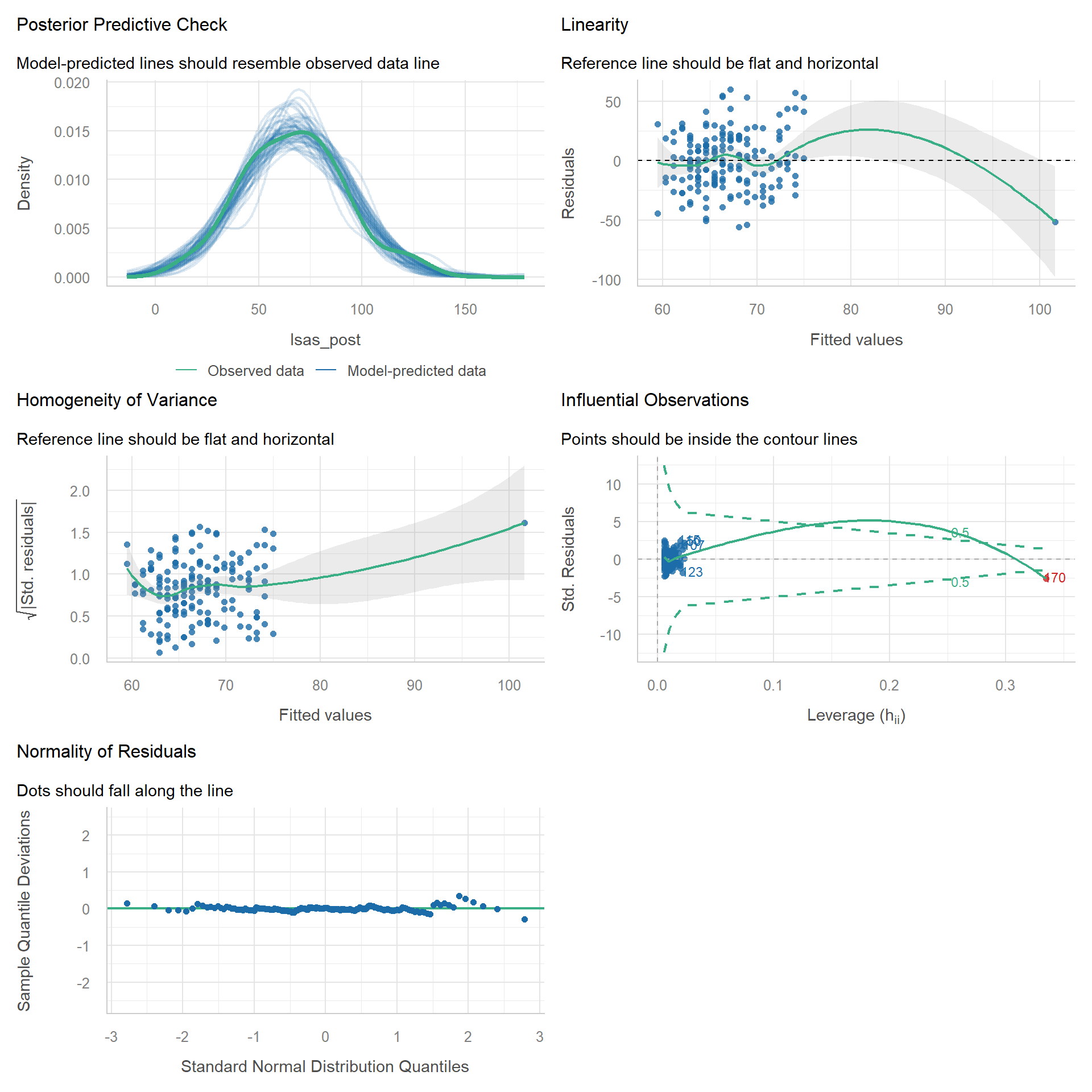
check_outliers(m_outlier)1 outlier detected: case 170.
- Based on the following method and threshold: cook (0.7).
- For variable: (Whole model).The extreme outlier is clearly visible on some of the plots, but note that it may not be apparent on the commonly used “Normality of Residuals” plot.
Non-Independent Errors (Therapist Effects)
Errors are assumed to be independent and have constant variance. A common violation of the independence assumption occurs when we take repeated measures on participants. However, longitudinal or timeseries data is not the focus of this course, so instead we will assume that participants are clustered (e.g., treated by the same psychotherapist). Patients who share the same therapist tend to have outcomes more similar than patients treated by another therapist. For example, if therapists have varying skills. This can also lead to correlated errors. Let’s simulate this: assume 10 therapists per treatment group, and each treats 50 patients (a nested design).
gen_therapist_data <- function(...) {
  n <- 50 # n per therapist
  n_therapists <- 20
  lvl2 <- rnorm(n_therapists, 0, 0.5)
  therapist_id <- rep(1:n_therapists, each = n)
  trt <- rbinom(n_therapists, 1, 0.5)
  epsilon <- rnorm(n * n_therapists, 0, 1)

  y <- 5 + 0.5 * trt[therapist_id] + lvl2[therapist_id] + epsilon
  data.frame(
    y,
    trt = factor(trt[therapist_id]),
    therapist_id = therapist_id
  )
}

d_therapist <- gen_therapist_data()
m_therapist <- lm(y ~ trt, data = d_therapist)
check_autocorrelation(m_therapist)
Warning: Autocorrelated residuals detected (p = 0.012).# Simulate
res3 <- run_sim(
gen_therapist_data,
formula = y ~ trt,
n_simulations = 500
)
sim_sum3 <- res3 |>
filter(Parameter == "trt1") |>
summarize(
est_mean = mean(Coefficient),
est_sd = sd(Coefficient),
se_mean = mean(SE),
CI_coverage = mean(CI_low <= 0.5 & CI_high >= 0.5)
)
sim_sum3| est_mean | est_sd | se_mean | CI_coverage |
|---|---|---|---|
| 0.51 | 0.25 | 0.07 | 0.45 |
Because we assumed a large therapist effect, the SEs are much smaller in the linear model that ignores clustering, and the confidence intervals include the true treatment effect in only 45% of simulations. This happens because the data generation treats therapists as a random factor: each therapist has a random effect drawn from a distribution, which induces correlation among patients of the same therapist and adds a therapist-level variance component. Ignoring this structure violates independence and typically underestimates SEs. To remedy this, use cluster-robust standard errors or fit a multilevel (random-effects) model with, for example, random intercepts for therapists.
NoteValidity, Representativeness and Fixed versus Random Effects
The clustering example illustrates issues of validity and representativeness, not just statistical assumptions. In our simulation, therapists are treated as a random factor: for each dataset, 20 therapist effects are drawn from a normal distribution. This induces within-therapist correlation and a therapist-level variance component.
However, fitting a random-effects model does not, by itself, make your study therapists representative of a wider population. Representativeness is a property of your sampling and study design, not the analysis model. Moreover, we might not want to generalize beyond the therapists in our study. From that perspective, the random-effects assumption may not match our research question. In this case, we could treat therapists as a fixed factor and condition on the therapists we include in our study. This reduces uncertainty about the treatment effect because we assume the therapists and their skill levels would be identical across hypothetical repetitions of our study. Neither perspective is right or wrong from a statistical perspective, it depends in what your inferential goals are.
Summary
In this chapter you learned:
- Run a quick diagnostic check with
check_model() - Diagnose and fix nonlinearity using polynomials and natural splines
- Detect heteroskedasticity
- Identify outliers and influence
- Non-independent errors