Chapter 4: Regression with a Numeric Predictor

1 Introduction

In the previous chapters, we studied regression models with:

• no predictors (intercept-only models)
• binary predictors
• categorical predictors with multiple levels

In this chapter, we move to a numeric predictor, called gad_screen.

Numeric predictors allow us to model continuous relationships, where the expected outcome changes smoothly as the predictor changes.

You will learn:

• how numeric predictors enter regression models
• how to interpret intercepts and slopes
• how linear regression models mean trends
• how quantile regression models quantile trends
• how to obtain predicted values across a range of the predictor
• how to visualize regression lines and uncertainty
• how to account for non-linear relationships between the predictor and the outcome

2 Packages and Data

library(tidyverse)
library(broom)
library(quantreg)
library(marginaleffects)
library(parameters)
library(here)

2.1 Load data

We will use gad_screen, a numeric measure of generalized anxiety symptoms at screening, as our predictor.

summary(df_clean$gad_screen)

   Min. 1st Qu.  Median    Mean 3rd Qu.    Max. 
   1.00    7.00   10.00   10.86   14.00   21.00 

3 Regression with a Numeric Predictor

With a numeric predictor, the regression model estimates:

1. the expected outcome when the predictor equals zero
2. the change in the outcome associated with a one-unit increase in the predictor

3.1 Model formula

lsas_post ~ gad_screen

This corresponds to the linear regression model for the conditional mean:

\[ \mathbb{E}(LSAS_{post,i} \mid gad\_screen_i) = \beta_0 + \beta_1\, gad\_screen_i \]

Where:

• \(\beta_0\) is the expected LSAS score when gad_screen = 0
• \(\beta_1\) is the expected change in the mean LSAS for a one-unit increase in gad_screen

For individual observations:

\[ LSAS_{post,i} = \beta_0 + \beta_1 \, gad\_screen_i + \epsilon_i \]

4 Linear Regression (Mean Trend)

4.1 Fit the model

mod_lm <- lm(lsas_post ~ gad_screen, data = df_clean)
summary(mod_lm)

Call:
lm(formula = lsas_post ~ gad_screen, data = df_clean)

Residuals:
    Min      1Q  Median      3Q     Max 
-65.031 -18.149   1.527  16.674  64.527 

Coefficients:
            Estimate Std. Error t value Pr(>|t|)    
(Intercept)  56.6502     4.8858  11.595   <2e-16 ***
gad_screen    0.9705     0.4171   2.327   0.0212 *  
---
Signif. codes:  0 '***' 0.001 '**' 0.01 '*' 0.05 '.' 0.1 ' ' 1

Residual standard error: 24.46 on 167 degrees of freedom
  (12 observations deleted due to missingness)
Multiple R-squared:  0.0314,    Adjusted R-squared:  0.0256 
F-statistic: 5.414 on 1 and 167 DF,  p-value: 0.02118

4.1.1 Interpretation

• (Intercept): expected mean at gad_screen = 0
• gad_screen: how much the mean LSAS score changes per unit increase in baseline anxiety

A positive slope indicates higher post-treatment LSAS scores among participants with higher baseline anxiety. For each one-unit increase in GAD-7 at screening, the expected mean LSAS at post increases by approximately 0.97 points.

4.2 Relationship to correlation

With a single numeric predictor, linear regression is closely related to Pearson correlation:

cor(df_clean$lsas_post, df_clean$gad_screen, use = "complete.obs")

[1] 0.1772046

In fact, if we standardize both the predictor and the outcome to z-scores with mean = 0 and SD = 1, the correlation and the coefficient will be almost identical with only one numeric predictor. This can be done using the scale() function within the regression:

coef(lm(scale(lsas_post) ~ scale(gad_screen), data = df_clean))[2]

scale(gad_screen) 
        0.1765964 

cor(df_clean$lsas_post, df_clean$gad_screen, use = "complete.obs")

[1] 0.1772046

Alternatively, we can also use the parameters-package to get standardized coefficients.

standardize_parameters(mod_lm, method = "basic") |> display()

# Standardization method: basic

Parameter	Std. Coef.	95% CI
(Intercept)	0.00	[0.00, 0.00]
gad screen	0.18	[0.03, 0.33]

5 Quantile Regression (Quantile Trends)

5.1 Model formulation

For quantile regression at quantile \(\tau\):

\[ Q_{LSAS_{post} \mid gad\_screen}(\tau \mid gad\_screen_i) = \beta_0(\tau) + \beta_1(\tau) \, gad\_screen_i \]

• \(\beta_0(\tau)\) = \(\tau\)-th quantile when gad_screen = 0
• \(\beta_1(\tau)\) = change in the \(\tau\)-th quantile per one-unit increase in gad_screen

5.2 Fit a median regression

mod_rq <- rq(lsas_post ~ gad_screen, tau = 0.5, data = df_clean)
summary(mod_rq)

Call: rq(formula = lsas_post ~ gad_screen, tau = 0.5, data = df_clean)

tau: [1] 0.5

Coefficients:
            coefficients lower bd upper bd
(Intercept) 61.72727     50.14774 74.72628
gad_screen   0.45455     -0.87730  2.38616

The slope now describes how the median LSAS score changes as baseline anxiety increases.

6 Predictions Using marginaleffects

With numeric predictors, predictions depend on the value of the predictor. We therefore compute predictions across a range of values.

6.1 Predicted means across gad_screen

# Create a grid of gad_screen values (50 points from min to max)
newdat <- datagrid(
  newdata = df_clean,
  gad_screen = seq(
    min(df_clean$gad_screen, na.rm = TRUE),
    max(df_clean$gad_screen, na.rm = TRUE),
    length.out = 50
  )
)

# Get predictions from the linear model at those values
pred_lm <- predictions(mod_lm, newdata = newdat)
pred_lm

gad_screen	Estimate	Std. Error	z	Pr(>|z|)	2.5 %	97.5 %
Type: response
1.00	57.6	4.50	12.8	<0.001	48.8	66.4
1.41	58.0	4.35	13.3	<0.001	49.5	66.5
1.82	58.4	4.20	13.9	<0.001	50.2	66.6
2.22	58.8	4.05	14.5	<0.001	50.9	66.7
2.63	59.2	3.90	15.2	<0.001	51.6	66.8
40 rows omitted	40 rows omitted	40 rows omitted	40 rows omitted	40 rows omitted	40 rows omitted	40 rows omitted
19.37	75.4	4.03	18.7	<0.001	67.5	83.4
19.78	75.8	4.19	18.1	<0.001	67.6	84.0
20.18	76.2	4.34	17.6	<0.001	67.7	84.7
20.59	76.6	4.49	17.1	<0.001	67.8	85.4
21.00	77.0	4.65	16.6	<0.001	67.9	86.1

The Estimate column shows the predicted mean value of lsas_post across a range of gad_screen values.

6.2 Predicted medians across gad_screen

pred_rq <- predictions(mod_rq, newdata = newdat)
pred_rq

gad_screen	Estimate	Std. Error	z	Pr(>|z|)	2.5 %	97.5 %
Type: response
1.00	62.2	6.97	8.92	<0.001	48.5	75.8
1.41	62.4	6.74	9.25	<0.001	49.2	75.6
1.82	62.6	6.51	9.60	<0.001	49.8	75.3
2.22	62.7	6.29	9.98	<0.001	50.4	75.1
2.63	62.9	6.06	10.38	<0.001	51.0	74.8
40 rows omitted	40 rows omitted	40 rows omitted	40 rows omitted	40 rows omitted	40 rows omitted	40 rows omitted
19.37	70.5	5.74	12.28	<0.001	59.3	81.8
19.78	70.7	5.97	11.85	<0.001	59.0	82.4
20.18	70.9	6.19	11.45	<0.001	58.8	83.0
20.59	71.1	6.42	11.08	<0.001	58.5	83.7
21.00	71.3	6.64	10.73	<0.001	58.2	84.3

The estimate column shows the predicted median value of lsas_post across a range of gad_screen values.

6.3 Marginal effect (slope)

For numeric predictors, contrasts correspond to slopes. These will be the same as the coefficient you got using the summary() function above.

avg_slopes(mod_lm)

Estimate	Std. Error	z	Pr(>|z|)	2.5 %	97.5 %
Type: response
0.971	0.417	2.33	0.02	0.153	1.79

For quantile regression:

avg_slopes(mod_rq)

Estimate	Std. Error	z	Pr(>|z|)	2.5 %	97.5 %
Type: response
0.455	0.62	0.733	0.463	-0.76	1.67

7 Visualization

We can now visualize the relationship using the predicted values we got using the predictions() function earlier. Remember that these were saved using in the objects pred_lm and pred_rq

7.1 Linear regression line with confidence interval

plot_predictions(mod_lm, condition = "gad_screen", points = 0.4) +
  labs(
    x = "GAD score at screening",
    y = "LSAS post-treatment",
    title = "Linear Regression: Mean LSAS vs Baseline Anxiety"
  ) +
  theme_minimal()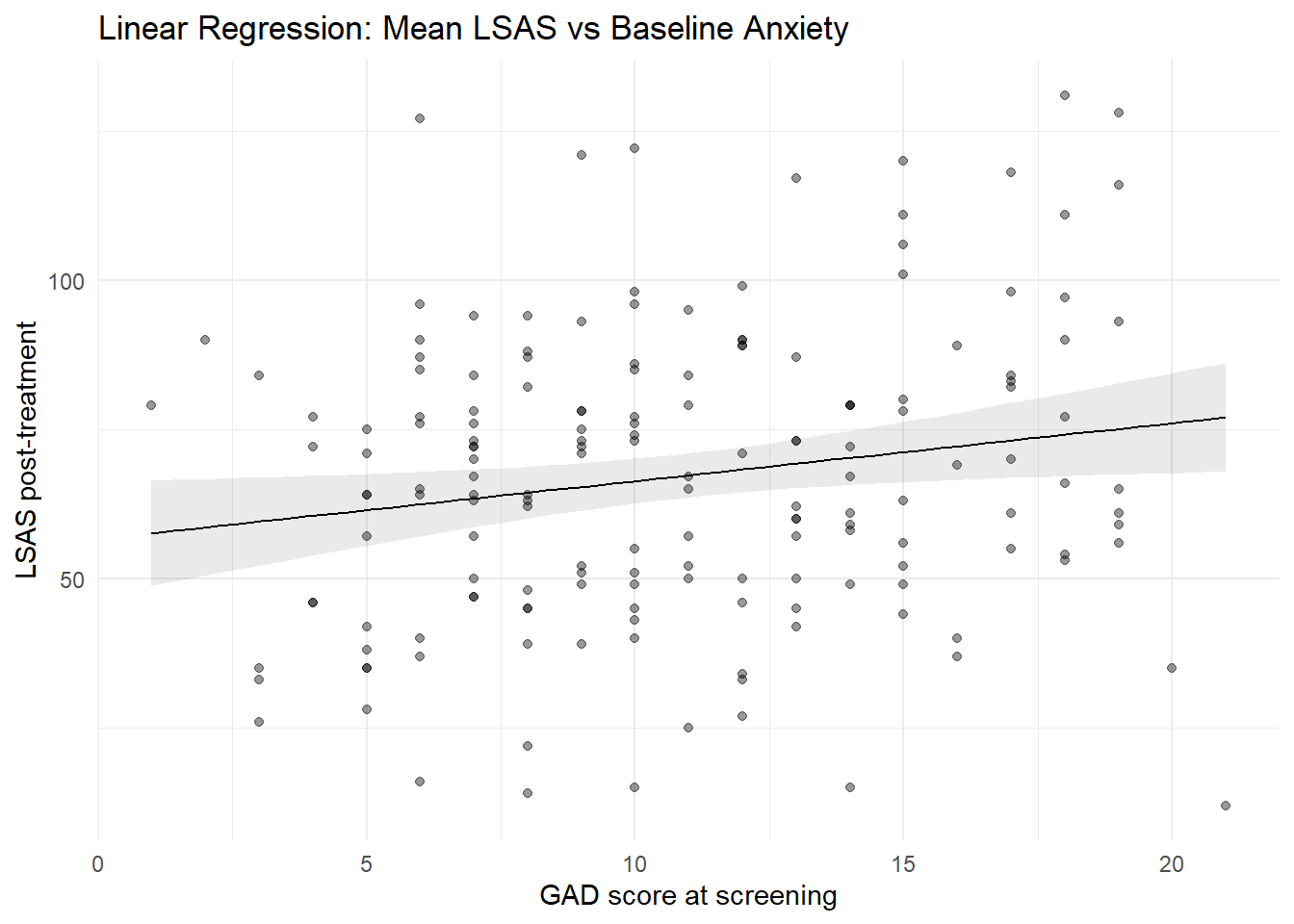

7.2 Median regression line with confidence interval

plot_predictions(mod_rq, condition = "gad_screen", points = 0.4) +

  labs(
    x = "GAD score at screening",
    y = "LSAS post-treatment",
    title = "Quantile Regression: Median LSAS vs Baseline Anxiety"
  ) +
  theme_minimal()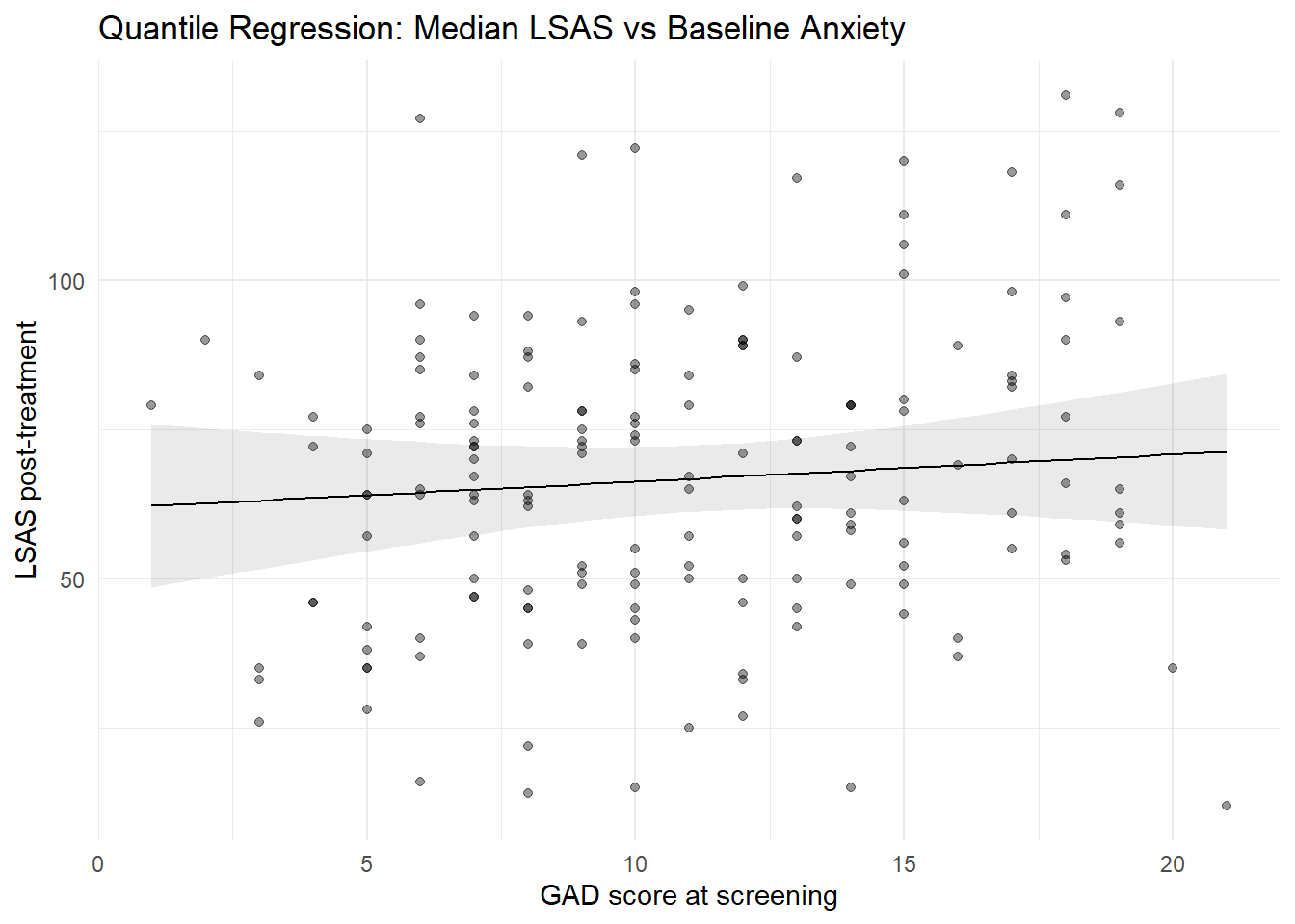

8 Modeling Non-Linear Relationships

So far, we have assumed that the relationship between baseline severity and post-treatment severity is linear.

However, clinical change processes are sometimes non-linear. For example:

• participants with very low baseline severity have limited room for improvement
• participants with very high baseline severity may show diminishing returns
• treatment effects may level off at the extremes

To explore this, we now examine the relationship between baseline LSAS score (lsas_screen) and post-treatment LSAS score (lsas_post).

In this section, we illustrate two common approaches to modeling non-linearity:

1. Polynomial regression
2. Spline regression

---

8.0.1 Polynomial regression

Polynomial regression models nonlinear relationships by adding powers of the predictor (e.g., quadratic, cubic), allowing the mean trend to deviate from straight line.

8.0.1.1 Model formulation

A quadratic polynomial model can be written as: \[ \mathbb{E}(LSAS_{post,i} \mid lsas\_screen_i) = \beta_0 + \beta_1 \, lsas\_screen_i + \beta_2 \, lsas\_screen_i^2 \]

This allows the relationship to be curved rather than straight.

8.0.1.2 Fit a quadratic model

In R, we use the poly() function. Setting raw = TRUE makes the coefficients correspond directly to powers of the predictor.

mod_lm_poly <- lm(lsas_post ~ poly(lsas_screen, 2, raw = TRUE), data = df_clean)
summary(mod_lm_poly)

Call:
lm(formula = lsas_post ~ poly(lsas_screen, 2, raw = TRUE), data = df_clean)

Residuals:
    Min      1Q  Median      3Q     Max 
-85.060 -12.942   3.565  13.443  42.811 

Coefficients:
                                    Estimate Std. Error t value Pr(>|t|)  
(Intercept)                       -43.518108  37.945495  -1.147   0.2531  
poly(lsas_screen, 2, raw = TRUE)1   1.753930   0.841860   2.083   0.0387 *
poly(lsas_screen, 2, raw = TRUE)2  -0.005122   0.004540  -1.128   0.2609  
---
Signif. codes:  0 '***' 0.001 '**' 0.01 '*' 0.05 '.' 0.1 ' ' 1

Residual standard error: 20.78 on 166 degrees of freedom
  (12 observations deleted due to missingness)
Multiple R-squared:  0.3048,    Adjusted R-squared:  0.2964 
F-statistic: 36.39 on 2 and 166 DF,  p-value: 7.875e-14

8.0.1.3 Interpretation

• The intercept is the expected LSAS score when lsas_screen = 0
• The linear term captures the overall trend
• The quadratic term captures curvature

Because individual coefficients are difficult to interpret, we rely on predicted values and visualization.

8.0.1.4 Visualizing the polynomial fit

plot_predictions(
  mod_lm_poly,
  condition = "lsas_screen",
  points = 0.4
) + labs(
  x = "LSAS score at screening",
  y = "LSAS post-treatment",
  title = "Polynomial Regression (Quadratic Relationship)"
) +
  theme_minimal()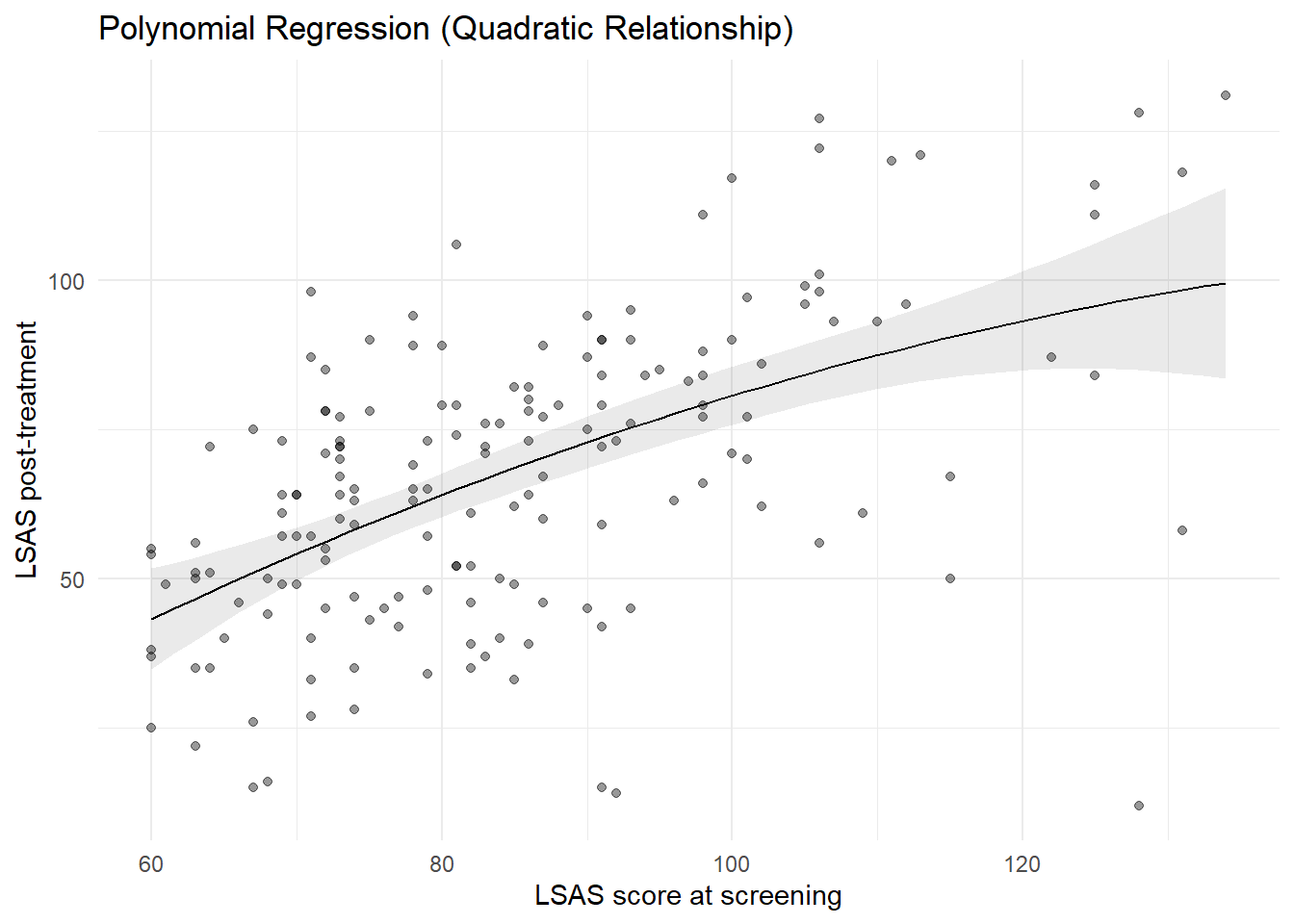

8.0.2 Spline regression

Polynomial models impose a global shape on the data. Spline regression offers a more flexible approach by fitting the relationship locally, while maintaining smoothness.

8.0.2.1 Model formulation

Using splines, the model is written as: \[ \mathbb{E}(LSAS_{post} \mid lsas\_screen) = \beta_0 + f(lsas\_screen) \] where \(f(\cdot)\) is a smooth function estimated from the data. In practice, splines approximate \(f\) with a set of piecewise cubic polynomials that are joined at a small number of locations called “knots.” The pieces are constrained to join smoothly, typically ensuring the function and its first two derivatives are continuous across knots. This allows the curve to adapt to local patterns without imposing a single global shape.

TipWhat is a natural cubic spline?

A natural cubic spline is a cubic spline with additional boundary constraints: outside the boundary knots, the function is constrained to be linear. This stabilizes the fit near the extremes of the predictor and reduces spurious wiggles in the tails. In R, splines::ns() can be used to constructs a natural cubic spline. You can control flexibility via either df or knots (internal knot locations). If knots is supplied, df is ignored.

• df: controls flexibility, e.g. how many knots that are used to construct the spline. With df and no knots, ns() places internal knots at equally spaced quantiles of the predictor within the boundary knots (by default the min and max).
• knots: Numeric vector of internal knot locations (on the predictor’s scale). When provided, ns() uses them exactly and ignores df. Use Boundary.knots to change the default min/max if needed.

So for ns(df_clean$lsas_screen, df = 4) we construct 4 columns, i.e. the model estimates four spline coefficients plus an intercept. This corresponds to a natural cubic spline with 2 boundary knots and 3 knots in-between.

8.0.2.2 Fit a spline model

library(splines)

mod_lm_spline <- lm(
  lsas_post ~ ns(lsas_screen, df = 4),
  data = df_clean
)
summary(mod_lm_spline)

Call:
lm(formula = lsas_post ~ ns(lsas_screen, df = 4), data = df_clean)

Residuals:
    Min      1Q  Median      3Q     Max 
-82.486 -12.822   2.455  13.112  45.024 

Coefficients:
                         Estimate Std. Error t value Pr(>|t|)    
(Intercept)                37.322      6.629   5.630 7.66e-08 ***
ns(lsas_screen, df = 4)1   19.444      7.546   2.577   0.0109 *  
ns(lsas_screen, df = 4)2   47.252      8.099   5.834 2.81e-08 ***
ns(lsas_screen, df = 4)3   82.116     16.089   5.104 9.13e-07 ***
ns(lsas_screen, df = 4)4   43.253      9.620   4.496 1.30e-05 ***
---
Signif. codes:  0 '***' 0.001 '**' 0.01 '*' 0.05 '.' 0.1 ' ' 1

Residual standard error: 20.62 on 164 degrees of freedom
  (12 observations deleted due to missingness)
Multiple R-squared:  0.324, Adjusted R-squared:  0.3075 
F-statistic: 19.65 on 4 and 164 DF,  p-value: 3.146e-13

As with polynomials, spline coefficients are not interpreted individually.

8.0.2.3 Visualizing the spline fit

knots <- ns(df_clean$lsas_screen, df = 4) |> attr("knots")

plot_predictions(
  mod_lm_spline,
  condition = "lsas_screen",
  points = 0.4
) +
  geom_vline(xintercept = knots, linetype = "dashed") +
  labs(
    x = "LSAS score at screening",
    y = "LSAS post-treatment",
    title = "Spline Regression (Natural Cubic Spline)",
    caption = "Vertical dashed lines show knots placement"
  ) +
  theme_minimal()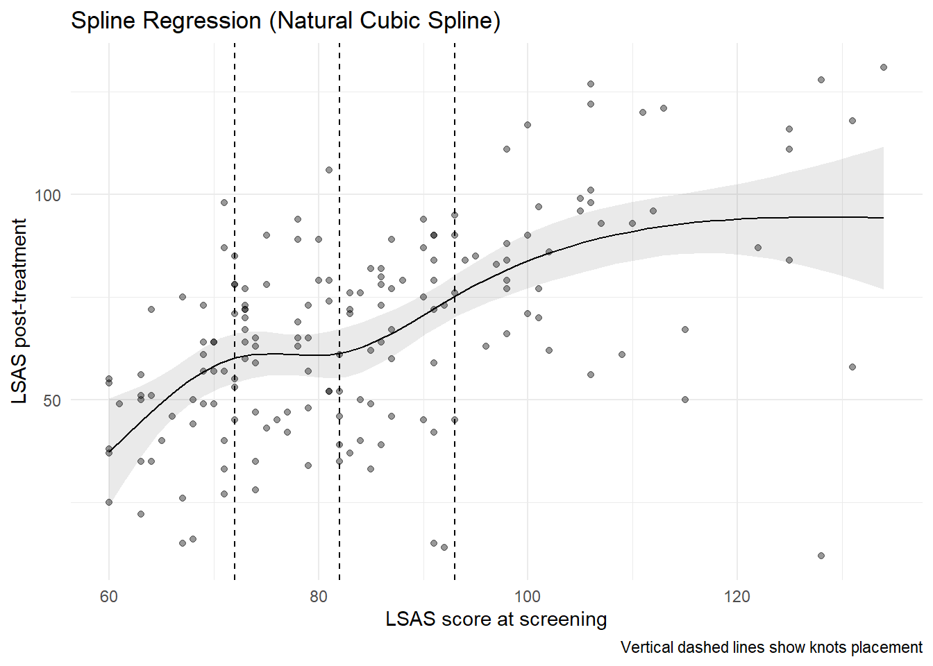

8.0.3 Comparing linear and non-linear fits

Finally, we compare:

• a linear model
• a quadratic polynomial model
• a spline model

mod_lm_linear <- lm(lsas_post ~ lsas_screen, data = df_clean)

# Grid for lsas_screen
newdat_lsas <- datagrid(
  newdata = df_clean,
  lsas_screen = seq(
    min(df_clean$lsas_screen, na.rm = TRUE),
    max(df_clean$lsas_screen, na.rm = TRUE),
    length.out = 100
  )
)

# Get predictions from each model
pred_linear <- predictions(mod_lm_linear, newdata = newdat_lsas) |>
  mutate(model = "Linear")
pred_poly <- predictions(mod_lm_poly, newdata = newdat_lsas) |>
  mutate(model = "Quadratic")
pred_spline <- predictions(mod_lm_spline, newdata = newdat_lsas) |>
  mutate(model = "Natural Cubic Spline")
# Combine into one data frame
pred_both <- bind_rows(
  pred_linear,
  pred_poly,
  pred_spline
)

# Plot
ggplot(df_clean, aes(x = lsas_screen, y = lsas_post)) +
  geom_point(alpha = 0.4) +
  geom_line(data = pred_both, aes(y = estimate, color = model), linewidth = 1) +
  labs(
    x = "LSAS score at screening",
    y = "LSAS post-treatment",
    title = "Linear vs Quadratic vs Spline Fits"
  ) +
  theme_minimal()

Warning: Removed 12 rows containing missing values or values outside the scale range
(`geom_point()`).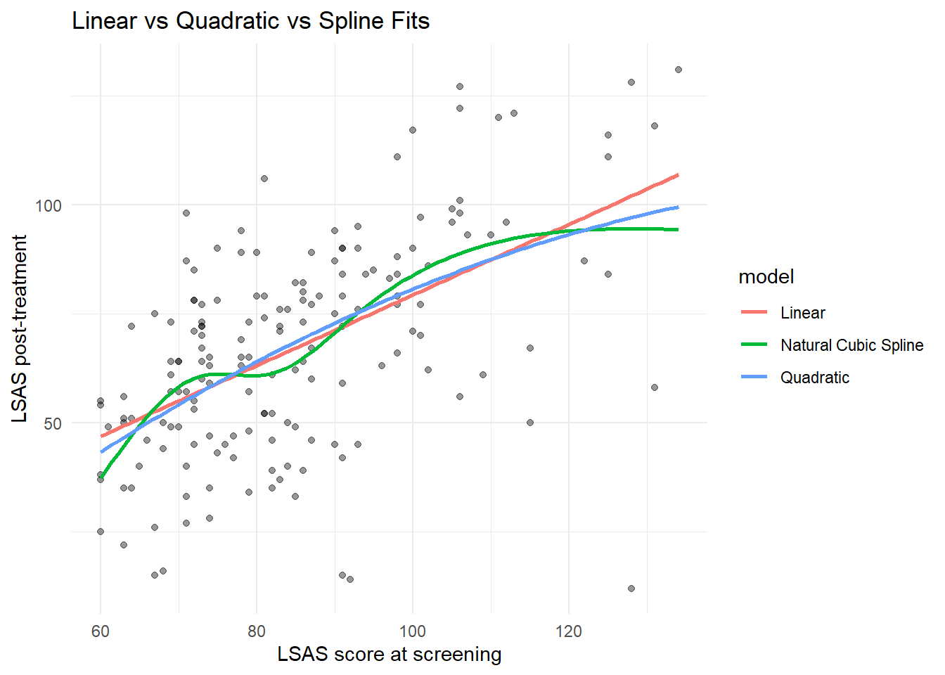

We can also formally compare the models.

# only for "nested" models
anova(
  mod_lm_linear,
  mod_lm_poly,
  mod_lm_spline
)

Res.Df	RSS	Df	Sum of Sq	F	Pr(>F)
167	72241.45	NA	NA	NA	NA
166	71691.76	1	549.692	1.293153	0.2571265
164	69712.93	2	1978.830	2.327603	0.1007432

performance::compare_performance(
  mod_lm_linear,
  mod_lm_poly,
  mod_lm_spline
) |> display()

Name	Model	AIC (weights)	AICc (weights)	BIC (weights)	R2	R2 (adj.)	RMSE	Sigma
mod_lm_linear	lm	1509.4 (0.37)	1509.5 (0.40)	1518.8 (0.86)	0.30	0.30	20.68	20.80
mod_lm_poly	lm	1510.1 (0.26)	1510.3 (0.27)	1522.6 (0.13)	0.30	0.30	20.60	20.78
mod_lm_spline	lm	1509.4 (0.37)	1509.9 (0.34)	1528.1 (8.00e-03)	0.32	0.31	20.31	20.62

When comparing, the differences between the non-linear fits and the straight line are small; non-linearities could arguably be ignored in modeling.

9 Summary

In this chapter you learned:

• how numeric predictors enter regression models
• how intercepts and slopes are interpreted
• how linear regression models mean trends
• how quantile regression models quantile trends
• how to compute predictions across a range of predictor values
• how to estimate and interpret marginal effects (slopes)
• how to visualize regression lines with confidence intervals
• how to allow for non-linear relationships

This chapter completes the foundation for regression models with a single predictor. In the next chapter, we will combine multiple predictors in the same model.