1 Introduction

In the previous chapter, we studied intercept-only regression models, which estimate a single summary of the outcome (a mean or a quantile).

In this chapter, we extend that framework by adding one binary predictor, called trt.

This is the simplest possible comparative regression model and corresponds to:

a two-sample t-test in linear regression
a comparison of quantiles in quantile regression

This chapter introduces how regression models encode group differences.

You will learn:

how binary predictors enter regression models
how to interpret intercepts and slopes with binary variables
how group means and differences are estimated
how to obtain predicted values for each group
how to visualize group comparisons
how linear and quantile regression differ in interpretation

2 Packages and Data

We use the same packages as before.

library(tidyverse)
library(broom)
library(quantreg)
library(marginaleffects)
library(here)

2.1 Load data

We load the same data as before.

df_clean <- read_csv2(here("data", "steps_clean.csv"))

We will use the treatment indicator variable trt as our predictor. In the original data, this indicator has three levels:

levels(as.factor(df_clean$trt))

[1] "self-guided"      "therapist-guided" "waitlist"

To get a binary variable (i.e., one with only two levels), we subset the data to include only participants in the therapist-guided or wait-list conditions. We’ll call this reduced dataset df_red.

df_red <- filter(df_clean, trt %in% c("therapist-guided", "waitlist"))

We transform the trt variable to a factor, and make sure that the wait-list condition is used as the reference.

df_red <- df_red |>
  mutate(trt = factor(trt, levels = c("waitlist", "therapist-guided")))

By listing wait-list as the first level, it becomes the reference level. We can check how R converts the factor to regression contrasts using contrasts.

contrasts(df_red$trt)

                 therapist-guided
waitlist                        0
therapist-guided                1

3 Regression with a Binary Predictor

With a binary predictor, the regression model estimates two quantities:

the expected outcome in the reference group
the difference between groups

3.1 Model formula

Here is the R syntax for the regression model for the LSAS post-treatment score, lsas_post, including only an intercept and the trt variable as a predictor (the intercept ~1 from the last model is implied, but can also be written out).

lsas_post ~ trt

lsas_post ~ 1 + trt

This corresponds to the linear regression model for the conditional mean:

\[ \mathbb{E}(LSAS_{post} \mid trt) = \beta_0 + \beta_1\, trt \]

Where:

\(\beta_0\) is the expected outcome when trt = 0 (waitlist group, since this is coded as the reference level)
\(\beta_1\) is the mean difference between the therapist-guided and waitlist groups (therapist-guided minus waitlist)

For individual observations:

\[ LSAS_{post,i} = \beta_0 + \beta_1\, trt_i + \epsilon_i \]

3.2 Interpretation of coefficients

trt	Predicted value
0 (waitlist)	\(\beta_0\)
1 (therapist-guided)	\(\beta_0 + \beta_1\)

Thus:

\(\beta_0\) = mean (or quantile) in the control group
\(\beta_1\) = difference in mean (or quantile) between the groups (i.e., treatment effect)

4 Linear Regression (Mean Differences)

4.1 Fit the model

mod_lm <- lm(lsas_post ~ trt, data = df_red)
summary(mod_lm)


Call:
lm(formula = lsas_post ~ trt, data = df_red)

Residuals:
    Min      1Q  Median      3Q     Max 
-64.448 -13.448  -1.948  12.624  62.648 

Coefficients:
                    Estimate Std. Error t value Pr(>|t|)    
(Intercept)           78.448      3.201  24.508  < 2e-16 ***
trttherapist-guided  -21.096      4.610  -4.576 1.25e-05 ***
---
Signif. codes:  0 '***' 0.001 '**' 0.01 '*' 0.05 '.' 0.1 ' ' 1

Residual standard error: 24.38 on 110 degrees of freedom
  (8 observations deleted due to missingness)
Multiple R-squared:  0.1599,    Adjusted R-squared:  0.1523 
F-statistic: 20.94 on 1 and 110 DF,  p-value: 1.25e-05

Interpretation

Intercept: estimated mean LSAS score in the control group
trt coefficient: estimated mean difference (therapist-guided minus waitlist). A negative value indicates lower mean LSAS at post in the therapist-guided group compared to the waitlist group. We can see that the mean value of LSAS at post was 21 point lower in the therapist-guided group than in the waitlist group.

We can verify these directly from the data:

df_red |>
  group_by(trt) |>
  summarize(mean_lsas = mean(lsas_post, na.rm = TRUE))

trt	mean_lsas
waitlist	78.44828
therapist-guided	57.35185

The difference between these two means equals the estimated coefficient for trt.

4.2 Relationship to the t-test

This regression model is mathematically equivalent to a two-sample t-test:

t.test(lsas_post ~ trt, data = df_red, var.equal = TRUE)


    Two Sample t-test

data:  lsas_post by trt
t = 4.5763, df = 110, p-value = 1.25e-05
alternative hypothesis: true difference in means between group waitlist and group therapist-guided is not equal to 0
95 percent confidence interval:
 11.96065 30.23220
sample estimates:
        mean in group waitlist mean in group therapist-guided 
                      78.44828                       57.35185

Regression generalizes the t-test by allowing:

additional predictors
non-normal outcomes
different estimands (e.g., quantiles)

5 Quantile Regression (Quantile Differences)

5.1 Model formulation

For quantile regression at quantile \(\tau\):

\[ Q_{LSAS_{post} \mid trt}(\tau \mid trt_i) = \beta_{0}(\tau) + \beta_{1}(\tau)\, trt_i \]

\(\beta_{0}(\tau)\) = \(\tau\)-th quantile in the control group
\(\beta_{1}(\tau)\) = difference in quantiles between groups

5.2 Fit a median regression

mod_rq <- rq(lsas_post ~ trt, tau = 0.5, data = df_red)
summary(mod_rq)


Call: rq(formula = lsas_post ~ trt, tau = 0.5, data = df_red)

tau: [1] 0.5

Coefficients:
                    coefficients lower bd  upper bd 
(Intercept)          77.00000     71.68339  84.63323
trttherapist-guided -24.00000    -31.77207 -16.61396

Interpretation is parallel to that for linear regression, but refers to quantiles instead of means. We can again verify group medians directly form the observed data:

df_red |>
  group_by(trt) |>
  summarize(median_lsas = median(lsas_post, na.rm = TRUE))

trt	median_lsas
waitlist	77.0
therapist-guided	52.5

6 Predictions Using `marginaleffects`

The marginaleffects package allows us to compute group-specific predictions. This allows us to see confidence intervals for the mean (or quantile) for each group, as well as the CI for the mean (or quantile) difference between the groups.

6.1 Predicted means by group (linear regression)

avg_predictions(mod_lm, by = "trt")

trt	Estimate	Std. Error	z	Pr(>\|z\|)	2.5 %	97.5 %
Type: response
waitlist	78.4	3.20	24.5	<0.001	72.2	84.7
therapist-guided	57.4	3.32	17.3	<0.001	50.8	63.9

This returns:

predicted mean in each group
standard errors
confidence intervals for each predicted mean

6.2 Predicted medians by group (quantile regression)

avg_predictions(mod_rq, by = "trt")

trt	Estimate	Std. Error	z	Pr(>\|z\|)	2.5 %	97.5 %
Type: response
waitlist	77	3.09	24.9	<0.001	70.9	83.1
therapist-guided	53	3.71	14.3	<0.001	45.7	60.3

6.3 Treatment effect as a contrast

avg_comparisons(mod_lm, variables = "trt")

Estimate	Std. Error	z	Pr(>\|z\|)	2.5 %	97.5 %
Type: response
-21.1	4.61	-4.58	<0.001	-30.1	-12.1

For quantile regression:

avg_comparisons(mod_rq, variables = "trt")

Estimate	Std. Error	z	Pr(>\|z\|)	2.5 %	97.5 %
Type: response
-24	4.83	-4.97	<0.001	-33.5	-14.5

6.4 Ratios

marginaleffects is highly flexible with regards to what hypothesis we can answer. For we example we can compare the ratio of mean outcomes.

# Mean ratio
hypotheses(
  mod_lm,
  hypothesis = "(`(Intercept)` + `trttherapist-guided`) / `(Intercept)` = 1"
)

Hypothesis	Estimate	Std. Error	z	Pr(>\|z\|)	2.5 %	97.5 %
(`(Intercept)`+`trttherapist-guided`)/`(Intercept)`=1	-0.269	0.0518	-5.2	<0.001	-0.37	-0.167

# Identical, but using b* syntax
hypotheses(
  mod_lm,
  hypothesis = "(b1 + b2) / b1 = 1"
)

Hypothesis	Estimate	Std. Error	z	Pr(>\|z\|)	2.5 %	97.5 %
(b1+b2)/b1=1	-0.269	0.0518	-5.2	<0.001	-0.37	-0.167

# Ratio of quantiles
hypotheses(
  mod_rq,
  hypothesis = "(b1 + b2) / b1 = 1"
)

Hypothesis	Estimate	Std. Error	z	Pr(>\|z\|)	2.5 %	97.5 %
(b1+b2)/b1=1	-0.312	0.0556	-5.61	<0.001	-0.421	-0.203

We can also change the reference level without having to refit the model (and much more).

avg_comparisons(
  mod_lm,
  variables = list(trt = c("therapist-guided", "waitlist"))
)

Estimate	Std. Error	z	Pr(>\|z\|)	2.5 %	97.5 %
Type: response
21.1	4.61	4.58	<0.001	12.1	30.1

6.5 Standardized Effect Sizes

If we want to report standardized mean differences (Cohen’s d), we can simply scale the estimates using an appropriate standardizer, for example the standard deviation at baseline.

sd_baseline <- sd(df_red$lsas_screen, na.rm = TRUE)

# Scale each estimate
smd <- avg_comparisons(
  mod_lm,
) |>
  mutate(
    estimate = estimate / sd_baseline,
    std.error = std.error / sd_baseline,
    conf.low = conf.low / sd_baseline,
    conf.high = conf.high / sd_baseline
  )
smd

Estimate	Std. Error	z	Pr(>\|z\|)	2.5 %	97.5 %
-1.17	0.256	-4.58	<0.001	-1.68	-0.671

# Equivalently, add standardization to hypothesis
avg_comparisons(
  mod_lm,
  variables = "trt",
  hypothesis = "b1 / 17.97963 = 0" # sd_baseline is 17.97963
)

Hypothesis	Estimate	Std. Error	z	Pr(>\|z\|)	2.5 %	97.5 %
Type: response
b1/17.97963=0	-1.17	0.256	-4.58	<0.001	-1.68	-0.671

7 Visualization

7.1 Group means with confidence intervals

Using marginaleffects::plot_predictions

plot_predictions(mod_lm, by = "trt") +
  labs(
    x = "Treatment group",
    y = "Estimated Mean LSAS (95% CI)",
    title = "Estimated Group Means from Linear Regression"
  ) +
  theme_minimal()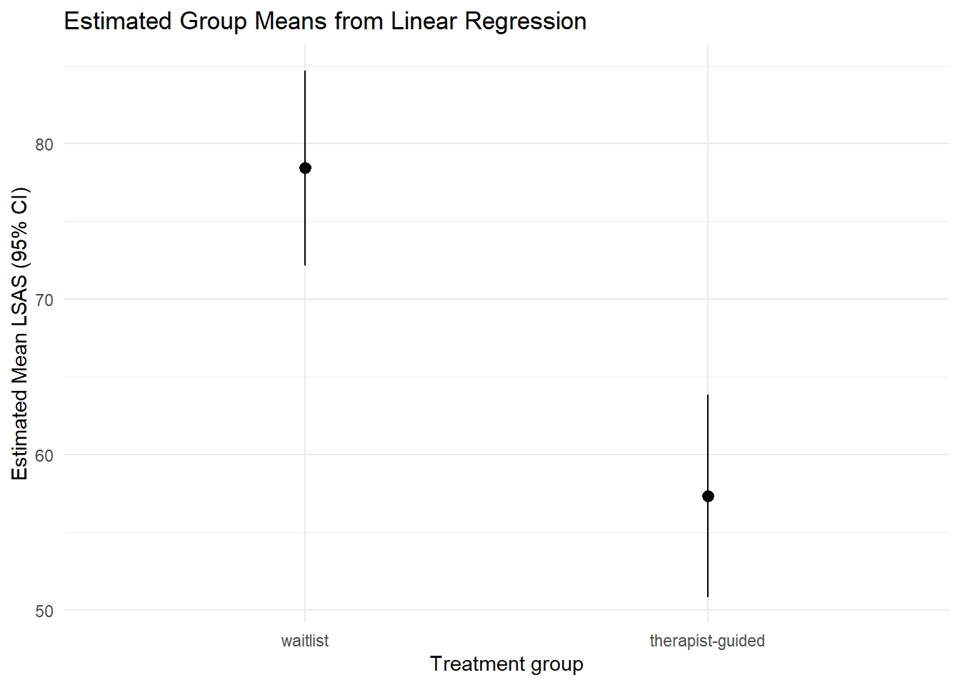

7.2 Group medians with confidence intervals

plot_predictions(mod_rq, by = "trt") +
  labs(
    x = "Treatment group",
    y = "Estimated Median LSAS (95% CI)",
    title = "Estimated Group Medians from Quantile Regression"
  ) +
  theme_minimal()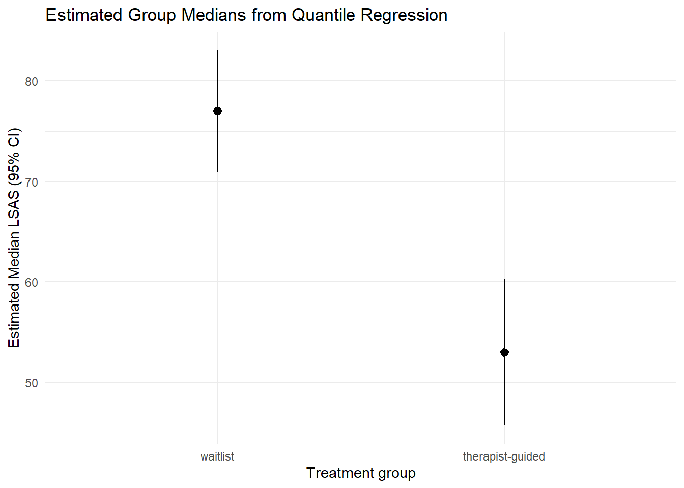

8 Summary

In this chapter you learned:

how binary predictors enter regression models
how intercepts and coefficients (slopes) encode group means and differences
how linear regression estimates mean differences
how quantile regression estimates quantile differences
how regression relates to t-tests
how to obtain predictions, contrasts, and confidence intervals
how to visualize group comparisons

This chapter provides the foundation for models with categorical predictors and later numeric predictors, and multiple predictors.