library(tidyverse)
library(here)
library(tinytable)

df_clean <- read_csv2(here("data", "steps_clean.csv"))Quarto Notebooks
Introducing notebooks
This chapter describes how to use Quarto notebooks to document your work. If you are familiar with things like Jupyter notebooks or R Markdown, Quarto works the same way. Notebooks are a type of document where you can mix text, code, and output. This is particularly helpful in projects that require statistical analysis, because you can keep everything in one place. We have found them to be useful in our own work, especially in the early stages of statistical analyses when we are trying to understand the data and need to explore different models and approaches. Is the concept of notebooks new? Then it might help to compare notebooks to other types of documents you are familiar with.
NoteThis website is built with Quarto
This entire course website is made up of Quarto notebooks. You can find the source code for this website in the lab-materials repository on GitHub.
Notebooks vs Word documents
When we write scientific manuscripts, we typically use something like Word to create the document. These often have options to insert tables, figures, and reference lists needed for the manuscript. One drawback of these documents is that they don’t handle code very well. You can’t run code in a Word file, and you can’t see the link between code and output. And when you need to update your manuscript with new results after making some adjustments, you need to manually enter the new results in tables and other parts of the document.
Notebooks combine code and output in a single document, so that any changes you make will be reflected in the output (figures, tables, etc). This means you avoid tedious manual work, and you lower the risk of errors from manual entry.
Notebooks vs .R scripts
R scripts are files of the type .R which contain code that you can run in R. They are the most straightforward way to write down your R code, but they are not the best way to document your work. Output is not saved in the script, and comments can only be added by adding # at the beginning of the line. As your R script becomes longer and longer, it is often difficult to keep track of everything going on.
An advantage of notebooks is that you can easily comment your code and discuss the results in the same place, and it is easy to add structure to your document by using headings, as well as referencing specific tables or figures by name.
Contents of a Quarto notebook
The typical Quarto notebook contains metadata, text and code. Metadata is provided on the first line of the notebook, and text or code is then added to the rest of the notebook, in any order you like.
Metadata
The first lines of a Quarto notebook are used to provide metadata about the notebook. This often includes the title of the notebook, the author, and the date of creation. The metadata is written in YAML format, and is enclosed in --- and --- lines.
(We added the date: last-modified option to automatically update the date of the notebook when you save it. This is helpful when you are sending around versions of your notebook to others.)
---
title: "Exploratory analyses"
author: "John Doe"
date: last-modified
---
Text
The text of a Quarto notebook is written in Markdown. Markdown is a lightweight markup language that is easy to write and read. It is a plain text format that can be converted to HTML, PDF, and other formats. For example, to make a heading you can use # at the beginning of the line. One # makes a first-level heading, two ## makes a second-level heading, and so on. To make the text bold, you use **bold text**. To make the text italic, you use *italic text*. To create a bullet point list, you use - at the beginning of the line. To create a numbered list, you use 1. at the beginning of the line.
Code
The code inside a Quarto notebook can be written in a variety of programming languages, but here we will use R. To write R code, you can type {r} to create a code chunk. For example, to run a simple R command, you can use:
two <- 1 + 1

two
[1] 2The code block is executed when the notebook is rendered, and the output is displayed below the code block. You can also run each code chunk individually by clicking the green play button in the top right corner. This is helpful when you are developing your code and want to test things as you go along.
NoteKeyboard shortcut to create a code chunk
In RStudio, you can use the keyboard shortcut Cmd + Opt + I to insert a new code chunk on Mac. This is a helpful shortcut to learn when working with Quarto notebooks!
Displaying output
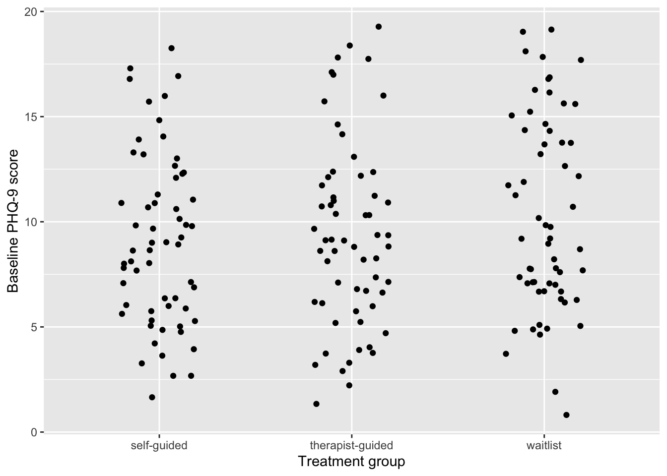
You can show plots and tables directly in your notebook. To enable direct references to the figure or table, you add some information at the beginning of the code chunk. Now when you reference @fig-phq9-screen, it will show Figure 1. And writing @tbl-phq9-screen gives us Table 1.
Text, code, and output all in the same place. This is why notebooks are great tools for statistical analysis.
df_clean |>
  ggplot(aes(x = trt, y = phq9_screen)) +
  geom_point(
    position = position_jitter(width = 0.2)
  ) +
  labs(
    x = "Treatment group",
    y = "Baseline PHQ-9 score"
  )
df_clean |>
  summarise(
    mean_phq9 = mean(phq9_screen, na.rm = TRUE),
    n = n(),
    .by = trt
  ) |>
tt()| trt | mean_phq9 | n |
|---|---|---|
| therapist-guided | 9.350000 | 60 |
| self-guided | 9.147541 | 61 |
| waitlist | 10.350000 | 60 |
Your task for the lab sessions
Your task for the lab sessions is to create Quarto notebooks to answer the questions. You can use the template notebook uploaded to Canvas as a starting point.
Where to get help
- Ask us!
- Check the chapters for course 2
- Check the Quarto documentation for help with Quarto